Futures Trend-Following Strategies

The core of this page comes from the book Following the Trend by Andreas F. Clenow.
Complementary notes, deep dives and references were added by me while reading the book.

Feel free to reach out to me with any comments, clarifications, or corrections.

Index

1. Introduction to Futures Contracts
2. Cross-asset trend following with futures
3. Futures data
4. Constructing diversified futures trading strategies
5. Two basic trend-following strategies

1. Introduction to Futures Contracts

We first spend some time introducing and defining futures contracts.

A futures contract is a standardized legal agreement to buy or sell a specific asset (underlying) at a predetermined price on a set date (delivery date) in the future.

In the futures market, exchanges set contract sizes, qualities, delivery dates and locations, so trades occur transparently and not OTC on organized exchanges (CME Group, ICE, Eurex). On the other hand, forward contracts or OTC derivatives can have similar characteristics but are traded over the counter as private, customizable and bilateral agreements without a settlement house or a central exchange.

The most important thing when entering a futures contract is that the trader doesn't have to pay the full contract upfront; he only posts an initial margin (typically 2 to 12% of the total underlying value) and then accounts are settled daily, i.e. profits or losses from the contract are credited or debited every day rather than waiting for expiration.

Daily PnL_{Long} = (F_{t} - F_{t - 1}) \times Contract Size

Daily PnL_{Short} = (F_{t - 1} - F_{t}) \times Contract Size

Furthermore, while holding a futures contract, the trader must have a maintenance margin, i.e. a minimum equity balance that must remain in the margin account. If this is violated, usually a margin call is issued and either additional deposits are requested or the position is liquidated.

At the delivery date $T$ , the futures price $F_{T}$ converges to the prevailing spot price $S_{T} = F_{T}$ , and so the cumulative profit or loss realized relative to the initial entry futures price $F_{0}$ is completely linear.

Π_{long} = S_{T} - F_{0}

Π_{short} = F_{0} - S_{T}

Futures Pricing Model: the "Cost of Carry" Framework

Futures prices are derived via the no-arbitrage pricing principle, i.e. the relationship between the spot price $S_{0}$ and the futures price $F_{0}$ is governed by the cost of carry ( $c$ ) that takes into account financing costs, storage costs and income yields.

In particular, for an asset with no holding costs or cash flows (i.e. non-dividend-paying stocks, gold as an investment, etc.) the fair futures price under continuous compounding is

F_{0} = S_{0} e^{r T}

where $S_{0}$ is the current spot price, $r$ the annualized risk-free rate and $T$ the time to maturity.

Indeed, if $F_{0} > S_{0} e^{r T}$ , an investor executes a cash-and-carry arbitrage by borrowing cash at rate $r$ , buying the spot asset at $S_{0}$ and shorting the futures contract at $F_{0}$ .

Similarly, if the asset yields a continuous income (a stock with dividend yield $q$ ), we have that

F_{0} = S_{0} e^{(r - q) T}

or, for some discrete income with present value $I$ , we have

F_{0} = (S_{0} - I) e^{r T}

For physical commodities, in the presence of storage costs $μ$ or convenience yield $y$ (the benefit of holding physical inventory during supply disruptions), both expressed as continuous rates, we have

F_{0} = S_{0} e^{(r + μ - y) T}

The Term Structure: Contango vs Backwardation

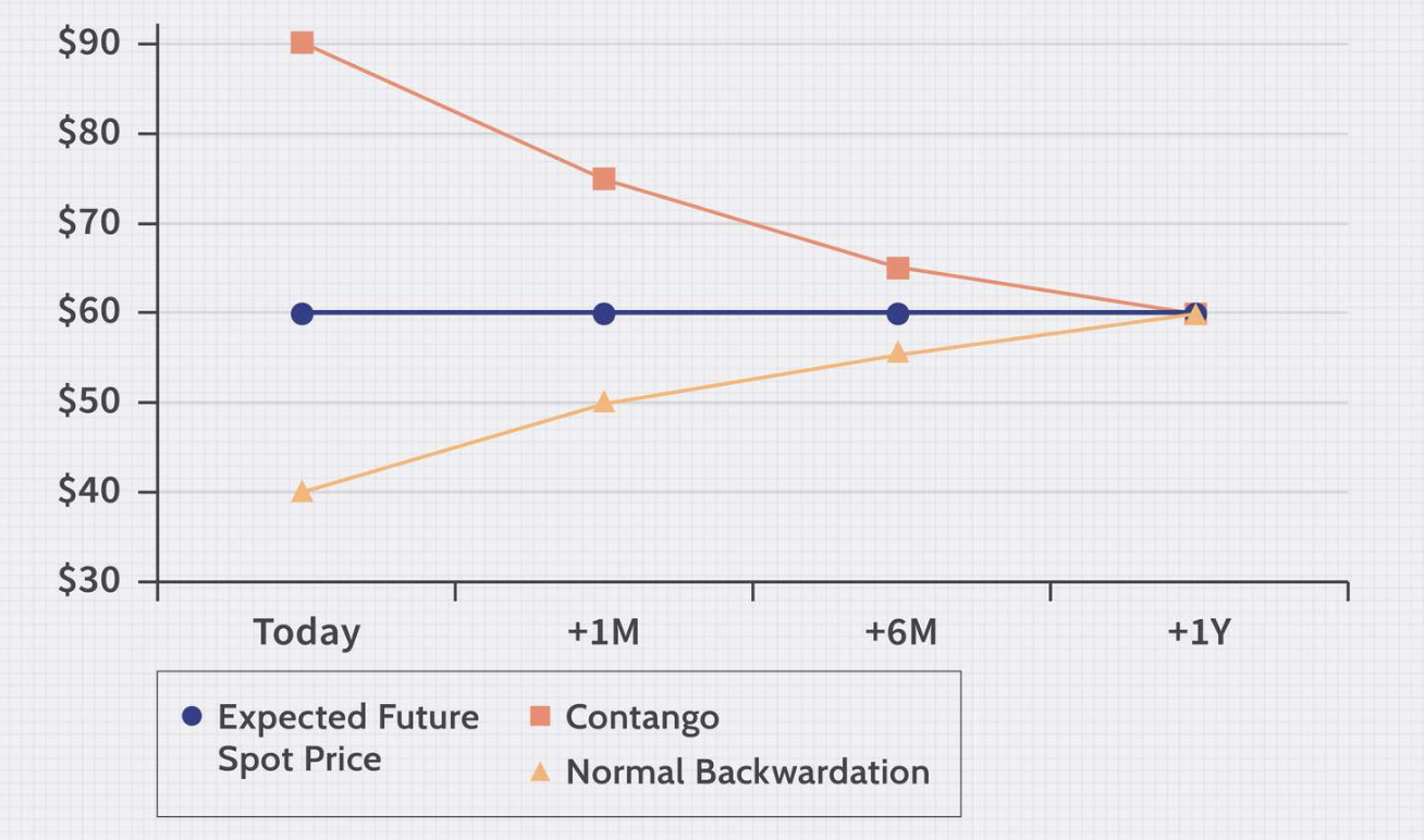
The relationship between spot prices and futures prices across different maturity dates brings us to the futures curve term structure, where we can distinguish two different market regimes.

Contango: $F_{0} > S_{0}$ (upward-sloping curve), when the carrying costs exceed the benefit of holding the asset ( $r + μ > y$ ), common in well-supplied commodity markets.
Backwardation: $F_{0} < S_{0}$ (downward-sloping curve), with high convenience yield ( $y > r + μ$ ) caused by immediate inventory shortages or high demand.

Bias variance tradeoff

Hedging Applications and Optimal Hedge Ratio

We first recall that hedging is implemented to reduce/remove an unwanted risk so that the outcome is more predictable. Note that hedging is not meant to make money; think of hedging as "insurance", where you give up some upside to limit the downside.

Cross-hedging happens whenever there are no futures contracts on the exact asset we want to hedge because, for example, there's no futures market, the contract doesn't match the exposure in size, location, or quality, it is not liquid enough or, in the case of portfolio-level hedging, we cannot hedge each stock's position.

In this case, we can offset price volatility in the underlying cash market position by minimizing the portfolio variance to obtain the optimal hedge ratio.

h^{*} = ρ_{SF} (\frac{σ _{S}}{σ _{F}})

where $ρ_{SF}$ is the correlation coefficient between spot price changes $Δ S$ and futures price changes $Δ F$ , and $σ_{S}$ and $σ_{F}$ are the corresponding standard deviations.

To derive the previous $h^{*}$ , consider the situation of a trader holding 1 unit of the spot asset and shorting $h$ units in futures.

The change in the portfolio is then

Δ V = Δ S - h Δ F

and we want $Δ V$ to be as stable as possible, so we minimize its variance:

Var (Δ V) = σ_{S}^{2} + h^{2} σ_{F}^{2} - 2 h Cov (Δ S, Δ F)

= σ_{S}^{2} + h^{2} σ_{F}^{2} - 2 h ρ σ_{S} σ_{F}

and, since this is convex in h, we can set the derivative to zero:

\frac{d Var}{d h} = 2 h σ_{F}^{2} - 2 ρ σ_{S} σ_{F} = 0

⟹ h^{*} = \frac{ρ σ _{S} σ _{F}}{σ _{F}^{2}} = ρ (\frac{σ _{S}}{σ _{F}})

If we plug $h^{*}$ back into the variance, we obtain the minimum variance as

Var_{m i n} = σ_{S}^{2} (1 - ρ^{2})

Once we have the optimal hedge ratio, we can calculate the optimal number of contracts.

Consider a portfolio with value $V_{A}$ and $V_{C} = F_{0} \times Q$ , the dollar value of one futures contract.

Consider then the P&L of the portfolio, defined as $Δ V_{A} = V_{A} r_{A}$ , and the P&L of the short futures position, $Q Δ F$ .

If we are short $N$ contracts on the futures, we have, using $Δ F = F_{0} r_{F}$ :

- NQ Δ F = - NQ F_{0} r_{F} = - N V_{C} r_{F}

We now consider $Δ V_{hedged}$ , the P&L of the hedged portfolio:

Δ V_{hedged} = V_{A} r_{A} - N V_{C} r_{F}

Also, we have $h = N V_{C} / V_{A}$ and $Δ V_{hedged} = V_{A} (r_{A} - h r_{F})$ .

If we now solve for N, we get:

N^{*} = h^{*} \frac{V _{A}}{V _{C}} = h^{*} \frac{V _{A}}{F _{0} Q}

Note that, in the case $h = 0$ , there's no hedge and the investor gets full $r_{A}$ . If $h = 1$ , the futures notional equals the portfolio value, so the investor is offset if $r_{A} \approx r_{F}$ .

2. Cross-asset trend following with futures

Most futures managers have done the same thing since 1970: trend following. The idea is very simple: use software to identify trends in a large set of futures markets, enter the trends and follow them as long as they last.

But..., even if they use sophisticated software and algorithms, the logic is simple and the strategies are not difficult to replicate. In reality, it is often not so easy to replicate them and make money.

The basic idea is that you never buy at the bottom and never sell at the top. Instead, you buy high and sell higher, or short low and cover lower, so you take the profits between the highest and lowest moment of the trend.

The underlying assumption is that financial markets tend to move in trends (perhaps not all the time and not even most of the time). Therefore, when markets are moving sideways, trend following is not profitable.

However, note that trend following on a single instrument is quite often a useless and very expensive exercise, since any single instrument can have very long periods where it does not work. Furthermore, trading on a single market or a few markets means taking too large bets.

Diversified futures strategies instead have the following characteristics:

large baskets of instruments to trade
coverage of all major asset classes
each bet is in itself almost insignificant compared to the total portfolio
most trend-following trades lose, but the idea is to gain more than what is lost on average.

Why diversified futures trends and why equities and bonds are not enough

Equities as an asset class have very high internal correlation, so they move together and diversification breaks down in market distress.
Equities move up in the long run, but we may not be able to afford their drawdown periods.

In contrast, managed futures usually show no correlation with equities, with a higher annualized compounded return and a lower drawdown.

Name	Annualised compound return (%)	Max DD (%)	Correlation to MSCI World	Annualised volatility	Starting date
MSCI World TR	8.1	−54.6		15.1	31 January 1988
Chesapeake Classic	10.1	−31.6	0.17	18.9	1 February 1988
Dunn World Monetary and Agriculture	12.9	−57.9	−0.09	32.1	1 November 1984
Eckhardt Evolution	10.9	−27.1	0.02	18.1	1 August 1991
EMC Classic	17.4	−45.4	−0.11	42.7	1 January 1985
Estlander Alpha	7.9	−29.7	0.04	13.6	1 October 1991
Fort Global Diversified	10.0	−17.5	−0.07	15.8	1 March 2002
ISAM Systematic Trend	11.2	−37.8	−0.20	18.2	1 June 2001
Mulvaney Global Markets	12.5	−45.1	−0.12	33.1	1 May 1999

Criticism of Trend-Following Strategies

survivorship bias, since some strategies did not survive or were closed. However, this is also true if we look at the performance of current S&P 500 companies... survivorship bias in finance is an extremely hard topic!
high leverage makes the strategy too risky. However, leverage and risk are not necessarily related.
trend following needs to short, and shorting has unlimited downside risk ...but you can only lose what you put on the table, so the loss is potentially unlimited only if you have unlimited margin capital, which is not the case.
managed futures funds have experienced large and long drawdowns. However, this is true for equities too (-55% for MSCI World in 2008).

But... note that:

managed futures strategies are scalable, since there is no downside in sharing the signal
you often need a large capital base to start trend-following trading, so aggregating resources and not trading from your private room makes sense.

But note that if you are trading someone else's money (i.e. if you run a fund), the performance may not be enough: you also need a good pitch and a good story to give a clear picture of what the fund does and why it could work (what the risk and return profile is, the backtest, which returns are targeted and so on), so work on presentation and marketing too.

Regarding this, pay attention not only to overall returns but in particular to drawdowns and volatility, since "volatility is the currency used to buy performance."

3. Futures data

With equities, if you buy some stocks quoted in USD but you do not earn/spend in USD, you are exposed both to the stock and to the currency. The return then depends both on the performance of the stock and on the currency.

With futures, the situation is different. When you open a futures position, no money changes hands except for commission fees. Since no money changes hands on initiation of the position, you have much less foreign exchange risk, and so your return depends on the currency exchange only when you close the position.

For example, suppose that you are CHF-based.

At $t = 0$ you buy 10 contracts of 10 Nasdaq Futures for 2,000 USD, with exchange rate 1.56.
You close the position at $t = 1$ by offsetting the contracts at a price of 1,834 USD.
You lose 166,000 USD, i.e. 166 basis points times the point value (in the case of Nasdaq, this is 100) times the number of contracts.
The exchange rate at $t = 1$ is 1.44.
So your loss in CHF is more or less 115,300, and the exchange rate at opening has no impact.

The currency exposure is not on the position but only on the P&L, and it varies day by day. It is both difficult to hedge but less impactful since it cannot change the direction/sign of the P&L.

Open Interest and Rolling

The open interest of a contract is the number of people actively trading it.

Most people in futures trading roll their positions, so open interest oscillates from month to month as people switch from one contract to another (with a longer expiry) as time goes on.

As a futures trader, you need a clear rule to switch from one contract to another. Common methods are based on volume and/or open interest.

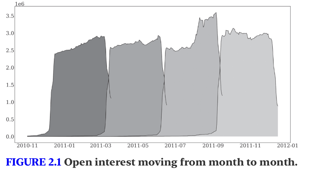
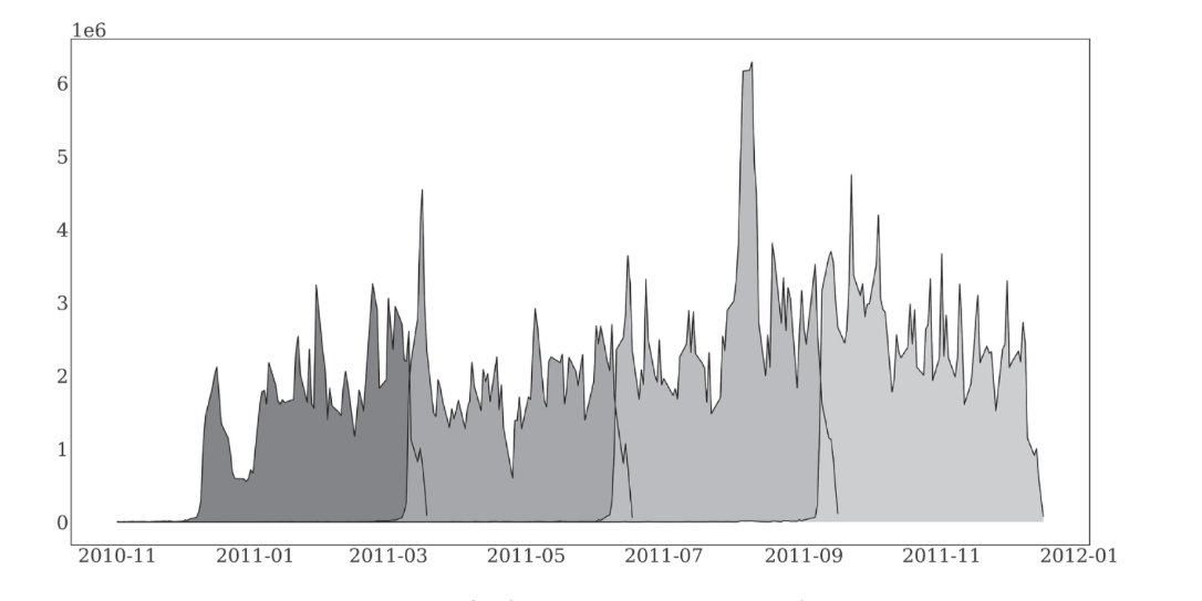
Open interest moving from month to month

Note that we often see volume spikes between months.

Volume across contract months

Term Structure

The term structure (or yield curve) refers to the shape of the curve obtained by plotting the delivery month on the x-axis and the futures price on the y-axis.

Term structure of heating oil

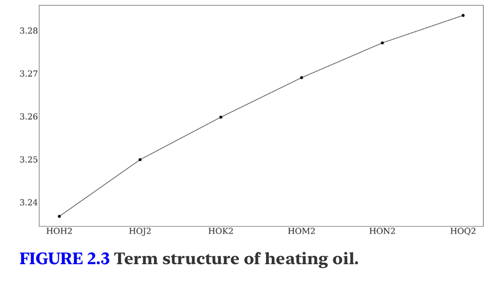
In the normal case, the price goes up in each successive month.

Upward slope: contango.
Downward slope: backwardation.

To understand why prices are higher in the future, we can think about the cost-of-hedging theory, which says that the fair price of any position is the cost of hedging it.

For example, suppose we want to buy 100 kg of gold in the future. The cost of hedging is the price of that gold plus the cost of storage, so the futures for longer months will be more expensive.

For financial futures there is no physical storage cost, so the interest rate is the main driver of the term structure:

the curve is less steep for financial instruments than for deliverable ones;
commodities with strong storage costs have a stronger term structure.

In contrast, note that backwardation is usually caused by seasonality, interest-rate conditions or an unusual storage-cost situation (not common for soft and perishable commodities).

Basis Gaps

The current prices of two contracts with the same underlying but different delivery dates will always be different and this difference is the basis gap.

The discrepancy comes primarily from hedging (carry) costs. This also creates a problem when we build continuous time series for long-term simulations using futures, since we cannot simply put one contract price series after another.

So we need to adjust the data. There are several ways to do it and the outcome is almost the same, but a common method is the following:

identify the liquid contracts based on open interest
link them together so that the old contract's close matches the new contract's close on the rollover date, keeping any gap at that time.

Note, however, that these continuations are not real and are not tradable instruments (they are not real price movements) and we should be aware of this while backtesting, since prices can be slightly different and considering that this hides rollover costs.

Futures Sectors

When dealing with futures...well, we could have a futures contract for each "real" object in the world... however, for simplicity, we briefly describe major futures sectors.

Agricultural commodities (lots of different products, from coffee and cotton to lean hogs or livestock... making it a very large supermarket)

internal correlation is not particularly high
all of them are affected by inflation to some degree
volatility can vary a lot since each contract is driven by fundamental developments; also news, adverse weather and seasonality play a big role
exchanges have so-called limit rules, i.e. a maximum price change in a single day
all futures are in theory deliverable, but for actual trading this is only an impossible theoretical scenario, because most brokers do not allow it
in agricultural commodities, small players have a big advantage since there are a lot of less liquid instruments with low correlation and they are liquid enough for trading accounts of a few tens of millions, but the big players cannot make profits because of their size.

Non-agricultural commodities (oil and its products)

they are highly volatile
they have high correlation with each other and they are prone to long-term trends $⟹$ this makes them suited for diversified futures trend following
Henry Hub (HH) natural gas is an interesting instrument since it is not usually highly correlated. Its contango is very large, since it is very expensive to store.
gold has value that is largely psychological and political, since it does not have a lot of industrial application. It is usually seen as a store of value and a protection against inflation, deflation, wars, riots and zombie attacks.
similarly, copper and silver have high correlation with gold and more industrial use.

Currencies (FX futures)

when you enter a currency futures contract, you are long one currency and short another
the currency market is the most liquid in the world
CTA funds tend to have large portions of their funds in currencies.
most of the currencies are quoted against the USD (if only one currency is named, it is against the USD).

Equities (single stocks and indices)

the largest futures market, with large internal correlation because individual cash equities have high internal correlation.
the unit used for equity index futures is points on the relevant index.
If you buy 5 contracts at 100 and sell them at 110, and the point value is 10, the gain is $(110 - 100) \times 5 \times 10 \times 1 = 500$ .

Rates (short-term interest rate futures, government bond futures)

the far left of the yield curve usually has lower price volatility than the far right, since these instruments have much lower duration and therefore less interest rate risk.

The point value is the dollar value of a move of 1 full point in the quoted futures price. It is set by the exchange for each contract (it is not a property linked to the asset) and it is usually computed as:

Point Value = \frac{Tick Value}{Tick Size}

or, when the contract has a size and a quoted price unit:

Point Value = Contract Size \times Price Unit

Similarly, for interest rate futures the Basis point value (BPV) is the dollar value of a move of 1 basis point (1 bp = 0.01% of the annualized rate) in the underlying rate. Since these contracts are quoted as

Futures Price = 100 - Annualized Rate

1 bp corresponds to a price move of $0.01$ full points, so

BPV = \frac{Point Value}{100}

Example (3-month Eurodollar future)

The Eurodollar is based on the three-month US dollar LIBOR (LIBOR has been discontinued and the contract replaced by the 3-month SOFR future, which has the same $25 per bp). The notional of this contract is USD 1 million. It is a bet on the 3-month interest rate, so a price of 98.00 means an implied rate of 2%.

Moving the price by 1 full point means that the rate moves by 1 percentage point, i.e. 1% per year. The contract only covers 3 months (1/4 of a year), so you earn a quarter of that:

convert the index point to a percentage by dividing by $100$ (1 index point = 1% of the annualized rate);
turn the annual rate into a quarterly one by dividing by $4$ .

Point Value = \frac{$1 , 000 , 000}{100 \times 4} = \frac{$1 , 000 , 000}{400} = $2, 500 per full 1.00 point

BPV = \frac{$2 , 500}{100} = $25 per basis point (bp)

This matches the tick value of the real contract.

If you hold a long position and the contract price moves from 98 to 99, the implied rate falls from 2% to 1%, i.e. $- 100$ bps (a price change of $+ 1.00$ full point), so

P&L = 1.00 point \times $2, 500 /point = 100 bp \times $25 /bp = $2, 500

...So long futures profit when rates fall.

Below find some typical examples:

Contract (ticker)	Contract size	Quoted in	Tick size = tick value	Point value
E-mini S&P 500 (ES)	$50 × index	index points	0.25 = $12.50	$50 per point
Micro E-mini S&P 500 (MES)	$5 × index	index points	0.25 = $1.25	$5 per point
E-mini Nasdaq-100 (NQ)	$20 × index	index points	0.25 = $5.00	$20 per point
Euro Stoxx 50 (FESX, Eurex)	€10 × index	index points	1 = €10.00	€10 per point
3-month SOFR (SR3)	$1,000,000	100 − annualized rate	0.0025 = $6.25	$2, 500 p er p o in t ($ 25 per bp)
10-year T-Note (ZN)	$100,000 face	% of par, in 64ths	1/64 = $15.625	$1,000 per point
Euro-Bund (FGBL, Eurex)	€100,000 face	% of par	0.01 = €10.00	€1,000 per point
EUR/USD (6E)	€125,000	USD per EUR	0.00005 = $6.25	$125,000 per 1.00
WTI crude oil (CL)	1,000 barrels	USD per barrel	0.01 = $10.00	$1, 000 p er$ 1.00
Natural gas (NG)	10,000 MMBtu	USD per MMBtu	0.001 = $10.00	$10, 000 p er$ 1.00
Gold (GC)	100 troy oz	USD per oz	0.10 = $10.00	$100 p er$ 1.00
Corn (ZC)	5,000 bushels	cents per bushel	0.25 cent = $12.50	$50 per 1 cent
Soybeans (ZS)	5,000 bushels	cents per bushel	0.25 cent = $12.50	$50 per 1 cent
Coffee "C" (KC, ICE)	37,500 lb	cents per lb	0.05 cent = $18.75	$375 per 1 cent
Sugar No. 11 (SB, ICE)	112,000 lb	cents per lb	0.01 cent = $11.20	$1,120 per 1 cent

4. Constructing diversified futures trading strategies

Note that there is a huge difference between understanding how to build a successful strategy and having the ability to thrive and the willpower to make it profitable in reality.

Note also that, if you plot the performance of the major managed futures funds in a time series:

on an absolute (unadjusted) basis they can look different;
but if you scale/normalize for volatility, they all look the same.

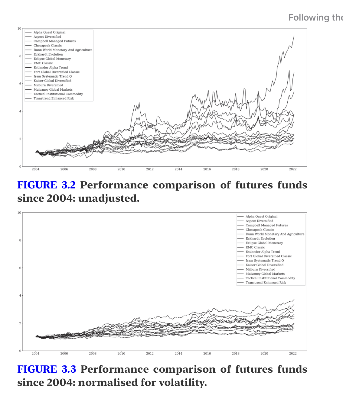
Performance comparison of futures funds, unadjusted and normalised for volatility

So, they are all doing the same thing!

Position Sizing

Which asset universe should we trade? There is always a trade-off between the number of markets and the complexity of the strategy.

More markets increase diversification and create more opportunities.
The exact number should depend on simulation and match the risk tolerance.

But... before any trading rules, you need a decent and concrete position-sizing formula.

Since different futures, depending on the underlying, show different volatility and therefore risk, we want to take the volatility of each instrument into account when deciding how many contracts to buy/sell. Most importantly, never put the same notional dollar amount in each trade.

The most common method is to take larger positions in less volatile assets, with the aim of having each position theoretically capable of making the same bottom-line profit/loss impact on the strategy.

In practice, we can use the average true range (ATR). It aims to measure how big a normal daily move is for each instrument and uses it as a starting point for position sizes.

T R_{t} = max (H_{t}, C_{t - 1}) - min (L_{t}, C_{t - 1})

where $H_{t}$ , $L_{t}$ and $C_{t - 1}$ are today's high, today's low and yesterday's close, so we arrive at the range in which we have been trading today. Then, for each day, we take the average of all $T R_{t}$ . Some common options include exponential smoothing.

The idea is that it provides not only a comparable number to standardize position sizes, but also an estimate of how large a move we can expect in a day.

We then use this information to set a target impact of the position on the portfolio. The target impact will become the leverage factor that we can scale up and down to shift the risk level.

The number of contracts can then be obtained as:

N = \frac{r \times E}{ATR \times PV}

where $r$ is the risk factor as a decimal (20 bp = 0.002), $E$ is the total equity and $P V$ is the point value.

Note that you could use volatility instead of ATR to estimate position sizing. In such case, let $σ_{d}$ be the daily volatility of returns (a decimal, e.g. 1% = 0.01), and $P$ the current futures price. The daily price move is $σ_{d} \times P$ , so:

N = \frac{r \times E}{σ _{d} \times P \times PV}

Note that the denominator $σ_{d} \times P \times PV$ is the daily dollar volatility of one contract (same role as $ATR \times PV$ before, so the formula is the ATR one with $ATR \approx σ_{d} \times P$ ).

For example, consider an initial risk factor of 20 basis points, so the theoretical average daily impact of each position should be 0.2%. Consider a portfolio of 1 million USD, so 0.2% translates to 2,000 USD. Suppose also that we receive a buy signal on gold and the ATR for gold at that time is 10 USD. Assuming that the gold contract has a point value of 100, each contract has a theoretical impact of USD 1,000. So, given our 2,000 USD target, we buy 2 contracts.

(Note that we used the term "theoretical" because volatility is not stationary and can change dramatically while holding the position.)

Furthermore, some hedge funds use margin-to-equity as their position sizing and risk measurement. In this case, the exchange sets the margins of each futures market based primarily on its view of volatility, to minimize the risk of default by market participants. The hedge fund then uses this as a basis, for example taking 0.5% of equity risk for each position, where equity is the full account value.

Trend Strategies

Looking at trend strategies, there are two common methods:

buying positive breakouts and shorting negative breakouts (you need to figure out what a breakout is);
using a classic trend indicator (moving average) and entering on different crossover rules. The simplest example is to plot a moving average, then buy if the price crosses above it and short when it crosses below.

Often, a filter rule is added on top, which allows you to enter the market long only when it is in a bullish phase, and vice versa for short positions. You want to avoid going accidentally against a strong trend just because of a short-term counter move. A good way is to combine two layers of trend measurement with different time horizons (a 200-day moving average and a shorter one for trend entry signals).

5. Two basic trend-following strategies

We now present 2 different trend-following strategies. Note that, even if they rely on different indicators, they can be combined and work better together.

Moving Average

The basis of this strategy is the moving average, i.e. the average price of the underlying in the last $x$ days. In particular, we consider 2 moving averages with different depths for the lookback period, so that we have a fast and a slow moving average.

(We can use different moving averages; the most common ones are the exponential ones over 50 and 100 days.)

The strategy goes both long and short and it is always in the market, i.e. for every asset in the asset universe (every futures contract) we are either long or short. The strategy is run on daily data and always trades the day after, to prevent look-ahead bias.

The logic is very simple: if the faster moving average is above the slower moving average, the trend is up, so we go long.

Breakout

The second strategy is still very simple: if today's closing price is higher than or equal to the highest close of the past 100 days, we buy the following day. Similarly, if the price is below or equal to the lowest close of the past 100 days, we sell at the open tomorrow and go short.

To get out of the position, a long trade is closed when the close reaches the lowest point in 50 days, and a short trade is covered when the price makes a 50-day high (always the day following the signal).

(Note that this strategy doesn't have to be always in the market.)

Performance

These strategies are quite uncorrelated with the MSCI World (and in general with equities):

when equities skyrocket, there is nothing we can do and the strategies look poor in comparison;
but the true value of these strategies is providing uncorrelated returns.

Also, note that the correlation between these two strategies has been fairly positive, and they have low correlation to the stock market.

The two strategies are more volatile than the benchmarks and show larger numbers in both return and risk (volatility). But note that volatility itself is not a risk, as it can be scaled up/down with the position-sizing factor.

Furthermore, note that the Sharpe ratio is not a meaningful metric here because:

it takes upward volatility into account as well, so for this we can use the Sortino ratio;
we are dealing with leveraged trading.

Combining the Strategies

The moving average strategy has the problem that it is always in the market, even if there is not really a trend. When there is sideways movement, the strategy tends to enter and exit after some time, losing each turn.

Conversely, the breakout strategy has the same problem: since it enters the market after seeing the highest/lowest price, it has the tendency to go against the main market trend at times.

The idea to solve both problems is to apply a trend filter to make sure we only trade in the direction of the main trend. We can indeed use the moving average for trend filtering and then use the breakout strategy for entries.

To sum up, the full strategy is:

broad universe of futures markets traded, across all major sectors;
trading daily;
trend is considered bullish if EMA 50 is above EMA 100;
trend is considered bearish if EMA 50 is below EMA 100;
enter long on a new 100-day high if the trend is bullish;
enter short on a new 100-day low if the trend is bearish;
exit long if the price falls to a 50-day low, or the trend turns bearish;
exit short if the price rises to a 50-day high, or if the trend turns bullish;
position sizing uses a 20-day ATR with a target of 15 basis points.

Cash Management

The interest rate is a very important factor in futures trading since, when dealing with futures, we do not need cash for our positions. We just need enough cash on the books to cover the initial margin and to avoid the risk of margin calls.

Note that when holding cash in a bank, we face counterparty risk, so we should carefully think about how to hold cash. An alternative is to stick with government debt of top-tier countries, preferably in your own currency.