"The aim of this course is to equip students with the skills to conduct simulations and perform mathematical convergence analysis for stochastic models, with applications in fields such as mathematical finance.
The course provides a comprehensive understanding of various numerical methods, covering their foundational principles, convergence properties, and practical implementation considerations." (from the official course's page)
The course has been taught at ETH Zurich by Professor Josef Teichmann and Dr Christoph Czichowsky.
Additional notes and notebooks can be found here.
Important remark: I do not take any credit for the content of the notes, all credit goes to the professor and their team!
Feel free to reach out to me with any comments, clarifications, or corrections.
Index
- 1. Basics of probability theory
- 2. Introduction to Stochastic Differential Equations
- 3. The Inversion Method
- 4. Monte Carlo Integration
- 5. Stochastic Integration and Itô Calculus
- 6. Stochastic Ordinary Differential Equations
- 7. Tractability
- 8. Strong approximation of Stochastic Differential Equations
1. Basics of probability theory
1.1. Probability foundations
Probability spacesA probability space is a mathematical concept that provides a formal model for a random experiment. It is composed of:
- sample space : the set of all possible outcomes.
- event space : the -algebra of subsets of . These subsets are called events, and they are the collections of outcomes to which we can assign probabilities.
- probability measure : a function that assigns a probability to each event. Note that satisfies the following:
- for all .
- .
- For any countable sequence of pairwise disjoint events , .
Expectation, Variance and Covariance
For a random variable , the expectation is the average value over a large number of trials.
If is discrete with probability mass function , we have:
If is continuous with probability density function :
For the same random variable , the variance measures the dispersion of values around the expected value, if it exists.
For two random variables , the covariance measures how they change together.
Note that variance and covariance have the following important properties:
- .
- .
- for constants .
- for constants .
- If and are independent, then ; the converse does not generally hold.
Furthermore, we can define the law of a random variable as the probability measure that satisfies , also called the pushforward measure.
Lastly, a fundamental concept in probability theory is independence: a family of random variables is called independent if the joint law of the family is the product of the marginal laws. In formulas:
The Law of Large Numbers (LLN)
The Law of Large Numbers states that, as the number of trials tends to infinity, the sample mean converges to the expected true value of the underlying distribution. Formally, we write:
Central Limit TheoremIt states that the distribution of sample means of a large number of independent and identically distributed random variables will be approximately normal, regardless of the original distribution of the random variables.
Conditional Probabilities and Laws
The conditional probability of given that event has occurred is:
For random variables, we can define conditional probability mass functions (PMFs) (for discrete variables) as:
and probability density functions (PDFs) for continuous variables as:
where is the joint PDF. If and are independent, .
Bayes' Formula
- is the posterior probability.
- is the likelihood, i.e. the probability of observing given that hypothesis is true.
- is the prior probability, i.e. the initial hypothesis of before any evidence.
- is the evidence (marginal likelihood), i.e. the total probability of observing .
- over all possible hypotheses .
Acceptance-Rejection Algorithm as Bayesian Reasoning
The Acceptance-Rejection (A-R) algorithm is a method for generating random samples from a target probability distribution using samples from a proposal distribution , especially when is difficult to sample directly.
This method can be viewed through a Bayesian lens, where the decision to accept or reject is observed data that updates our belief about whether the sample comes from the target distribution.
We then consider:
- prior-proposal: the samples drawn from the proposal distribution as realizations of (we are proposing that might also be a sample from after accepting/rejecting)
- likelihood/acceptance criterion: generate an independent uniform random variable , and accept if:
where is a constant such that . Note that the acceptance criterion is our data that helps us decide whether we accept samples from as samples from law .
- posterior: if a sample is accepted, it means that we have updated our belief such that this is a valid sample from . Iterating the process ensures that we accept only samples distributed according to .
Then, assume random variables live on a probability space with measure .
We first calculate the relevant quantities:
- is the set of accepted sample events, i.e. , with
- this allows us to calculate the law of posterior under acceptance, that is:
That means that, conditional on , the random variable , unconditionally -distributed, is actually -distributed.
Monte Carlo Integration (Corollary of LLN and CLT)
Monte Carlo integration is a numerical method for approximating the value of a definite integral, especially in the multidimensional case or over complex domains, by using the Law of Large Numbers.
We first consider the integral , which can be rewritten as:
where (uniformly distributed on ). Thanks to the LLN, we can approximate by averaging many samples of , so the integral becomes:
In this case, the CLT states that the error scales as .
Pseudo-Random Number Generators (PRNGs) vs True Random Number Generators (TRNGs)
Whenever we use Monte Carlo integration, we need a sequence of samples of random variables. To generate them, we can consider:
-
Pseudo-Random Number Generators (PRNGs):
- deterministic algorithms that produce sequences of apparently random numbers but are determined by an initial value called a "seed" (given the same seed, a PRNG gives the same sequence)
- they are fast, efficient and, most importantly, reproducible
- however, their deterministic nature makes them unsuitable for applications that require true randomness (e.g. cryptography)
-
True Random Number Generators (TRNGs)
- they extract randomness from physical phenomena (e.g. atmospheric noise, thermal noise in resistors, etc.)
- they are slower and often require specialized hardware
Formally, we can say:
Let be a probability space and let , for , be a sequence of -independent -distributed random variables.
-pseudo-random numbers are sequences of real numbers calculated by a deterministic algorithm that have similar statistical properties to .
Even if this is a very generic definition, the importance and advantage of -pseudo-random numbers are that they can be reproduced many times (with the same output) with the same pseudo-random input.
1.2. Sampling and random numbers
2. Introduction to Stochastic Differential Equations
2.1. Financial and physical stochastic models
We first show three important examples of stochastic differential equations, largely discussed in the sector and for which numerical approximations will be useful.
The Black–Scholes Model
Before starting: quick history recap: The Black–Scholes Model was initially published in 1973 by the economists Black and Scholes, based on a previous mathematical formulation by Merton. The model revolutionized modern finance by providing the first framework for pricing options. Curiously, the publication date (1973) coincided with the opening of the Chicago Board Options Exchange (CBOE, which is still active and covers approximately 30% of total option trading volume per year), which provided the first centralized marketplace for trading options.
From the model, we can deduce the Black–Scholes formula, which returns the theoretical value of the price of a European option (recall that a European option can be exercised only at maturity, while an American option can be exercised anytime).
The model assumes that the price of the underlying asset follows a geometric Brownian motion (GBM, one of the most important stochastic models in financial economics) and [... place other assumptions]
We begin by drawing the trajectory of a Brownian motion in Python.
import numpy as np
import matplotlib.pyplot as plt
# Parameters for Brownian Motion
T = 1.0 # Total time
N = 1000 # Number of steps
dt = T / N # Time step size
# Generate a Brownian Motion trajectory
np.random.seed(42) # for reproducibility
# Generate N independent increments
dW = np.random.normal(loc=0.0, scale=np.sqrt(dt), size=N)
W = np.cumsum(dW)
t = np.linspace(0, T, N)In the code: we first generate independent increments with mean and standard deviation. Secondly, we build the Brownian motion by cumulative sums.
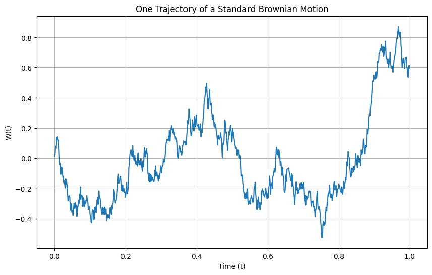
Formally, we can write:
where
- is the stock price at time .
- is the drift coefficient (the expected log return).
- is the volatility (standard deviation of log returns).
- is a Wiener process (Brownian motion).
Recall that is a stochastic process that satisfies:
- almost surely.
- It has independent increments for : .
- Its paths are almost surely continuous.
Therefore we have:
The equation should be understood as a (stochastic) integral equation.
Intuition: the equation says that the infinitesimal increment at time is approximately normally distributed with variance and mean .
In Python, we can write:
# Parameters for Black-Scholes simulation
S0 = 100 # Initial stock price
mu = 0.05 # Drift (expected return)
sigma = 0.20 # Volatility
T = 1.0 # Total time
N = 1000 # Number of steps
dt = T / N # Time step size
# Generate a single trajectory of stock prices
np.random.seed(42) # for reproducibility
S = np.zeros(N)
S[0] = S0
for i in range(1, N):
dW = np.random.normal(loc=0.0, scale=np.sqrt(dt))
S[i] = S[i-1] * np.exp((mu - 0.5 * sigma**2) * dt + sigma * dW)
t = np.linspace(0, T, N)
Langevin Equation (Simplified SDE)
The Langevin equation was inspired by the dynamics of a particle in a potential, where the gradient of the potential determines the force acting on the particle. It is the theoretical foundation of highly influential algorithms like Markov chain Monte Carlo or stochastic gradient descent. The goal of the equation is to sample from .
Recall, a potential function is a scalar function that defines the drift through its scaled negative gradient:
where is the drift function, i.e. the deterministic instantaneous tendency of the process in its state .
In general, for a in one dimension, the stochastic differential equation is given by:
where
- is the position of the particle at time .
- is the potential energy function.
- is the derivative of the potential with respect to .
- is a parameter related to noise.
- is Brownian motion.
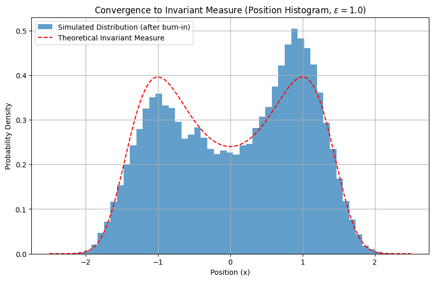
Note that the process converges in distribution to an invariant measure given by the density with respect to Lebesgue measure, i.e. solving the differential equation for large times brings samples of the invariant measure:
Recall that the invariant measure is a probability distribution that remains unchanged under the evolution of a stochastic process. Formally, if , then for all and, intuitively, it is the process's stationary theoretical distribution (long-run distribution).
In Python, we write the following:
# Parameters for Langevin SDE
dt = 0.01 # Time step
T = 500 # Total simulation time
N = int(T / dt) # Number of steps
epsilon = 1.0 # Noise intensity parameter
# Define a potential function (e.g., a double well potential)
def potential(x):
return 0.5 * (x**2 - 1)**2
def grad_potential(x):
return 2 * x * (x**2 - 1) # dU/dx
# Initialize position
x = np.zeros(N)
x[0] = 0.0
# Simulate Langevin dynamics using Euler-Maruyama
for i in range(N - 1):
dW = np.random.normal(loc=0.0, scale=np.sqrt(dt))
x[i+1] = x[i] - 0.5 * grad_potential(x[i]) * dt + np.sqrt(epsilon) * dW
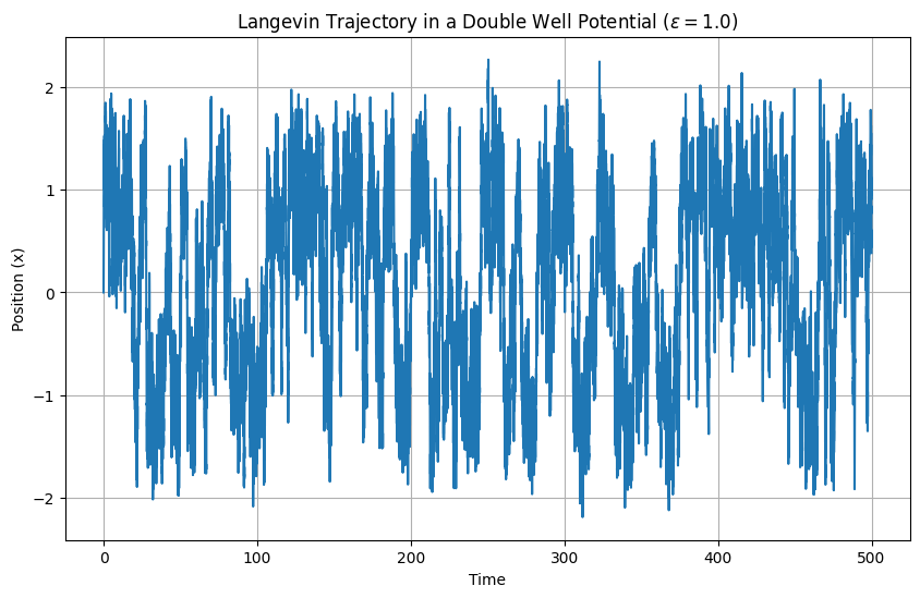
Furthermore, in the following plot we can see the convergence of the simulated distribution to the theoretical invariant measure.
2.2. Filtering and noisy observations
The Kalman Filter (Continuous Time for OU Process)The Kalman filter provides an optimal estimate of the state of a linear system observed with additive Gaussian noise.
Intuition: the filter repeats two steps:
- use the dynamics to predict the following state
- compare the prediction with the new observation and combine them, giving more weight to whichever is more reliable.
We now illustrate the filter with an Ornstein–Uhlenbeck process, which describes a mean-reverting particle with white noise, with the following SDE:
where is the long-run mean and is the reversion speed
We now consider a noisy observation of this OU process.
In this case, we observe such that , where are independent random variables with representing the measurement noise.
Intuition: in an OU process, is hidden and we only see the noisy signal, with as the unobserved OU state, as the observation, and as the noise.
Over a short interval , we can say:
where represents the standardized measurement noise in the discretized observation.
dt_sim = 0.01 # Simulation time step
T_sim = 100 # Total simulation time
N_sim = int(T_sim / dt_sim)
theta = 0.1 # Reversion speed
mu_ou = 0.5 # Mean
sigma_ou = 0.2 # Volatility
np.random.seed(43) # for reproducibility
X_true = np.zeros(N_sim)
X_true[0] = 0.0 #initialize at zero
for i in range(N_sim - 1):
# wiener process
dW = np.random.normal(loc=0.0, scale=np.sqrt(dt_sim))
# sde
X_true[i+1] = X_true[i] + theta * (mu_ou - X_true[i]) * dt_sim + sigma_ou * dW
t_sim = np.arange(N_sim) * dt_sim
# we now generate noisy observations
obs_noise_std = 0.5 # std of observation noise
R_obs = obs_noise_std**2 # variance of noise variance
# we sum up the simulated x_t and the noise
Z_obs = X_true + np.random.normal(0, obs_noise_std, N_sim)
We now spend some time explaining the Kalman filter.
Given and , we can introduce the Kalman filter with the following parameters:
- : mean-reversion coefficient
- : intensity of the process noise
- : variance of the Brownian noise
- : observation coefficient
- : variance of the observation noise Formally, we write:
that, for this scalar OU model, translates to
Then, using Euler's method, we can approximate:
where is the uncertainty before using the following observation.
Then, we can still use the Euler approximation with for the following expression:
The Kalman gain determines how much we can trust the new observation (large gain: we can trust it more) and is defined as:
Lastly, we update the state with:
(the term in parentheses represents the innovation or prediction error, i.e. the difference between the observation and the value predicted by the model)
Starting from the previous code block, we can implement the Kalman filter as:
# we now apply the Kalman Filter
# System parameters for Kalman Filter
F = -theta
L = sigma_ou
Q_process = 1.0 # Covariance of dW (in the case of unit variance)
H = 1.0
R_measurement = R_obs
dt_filter = dt_sim # Use the same time step for filter discretization
# initial conditions for Kalman filter
x_hat = np.zeros(N_sim)
P = np.zeros(N_sim)
x_hat[0] = Z_obs[0] # Initialize estimate with first observation
P[0] = 1.0 # Initial covariance (high uncertainty)
for k in range(N_sim - 1):
# Prediction step
P_minus = (1 + F * dt_filter)**2 * P[k] + L**2 * Q_process * dt_filter
x_hat_minus = x_hat[k] + theta * (mu_ou - x_hat[k]) * dt_filter
# Kalman gain
K_k = P_minus * H / (H * P_minus * H + R_measurement)
# Update step
x_hat[k+1] = x_hat_minus + K_k * (Z_obs[k+1] - H * x_hat_minus)
P[k+1] = (1 - K_k * H) * P_minus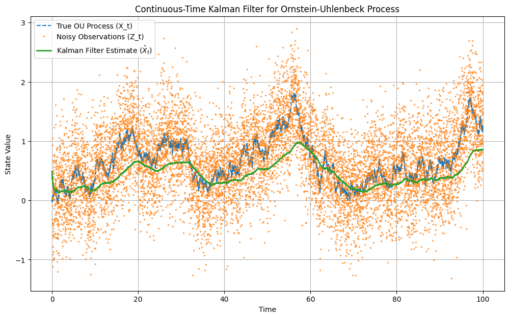
3. The Inversion Method
3.1. Generalized inverse distribution functions
Method for General Distributions Inversion MethodWe now spend some time presenting the inversion method, useful for transforming uniformly distributed random numbers into arbitrary distributions using a suitable generalized inverse distribution function.
Definition (Generalized inverse distribution function associated to a distribution function)Let be a distribution function. We define the generalized inverse distribution function associated with , denoted as , as the function which satisfies, for all , the following:
The crucial switching formula is:
From the definition, we can draw some nice properties:
- For all , the set is not empty and bounded from below.
- (This comes from the fact that, given , for all the set is not empty.)
- The fact that ensures that the set is bounded from below.
- is also sometimes referred to as the quantile function associated with .
- Consider a probability space and , an -measurable function (imagine as a model for the change in value of a financial portfolio).
Consider , the distribution of , and let be a confidence level, typically a number close to 1 (95%, 99.999%): Then the real number
is called the Value at Risk with confidence level associated with (i.e. it holds with probability of at least that the loss does not exceed ).
Theorem: The Inversion Method
Let and assume almost surely. Then has distribution function .
ProofFor every , the switching formula gives:
because is uniform on . Intuition: to sample from an arbitrary one-dimensional distribution, we can simply sample one uniform random variable and apply the quantile function to the sample.
Lemma (Properties of generalized inverse distribution functions)
Let be a distribution function and the generalized inverse distribution function associated with . Then fulfils the following:
- is non-decreasing.
- For all :
- .
- .
- .
- For all : .
- For all , : if and only if (switching formula).
- For all , : if and only if (switching formula).
- For all open sets with the property that is injective and all , we have that .
(Recall: a function is injective if implies ; equivalently, distinct inputs have distinct outputs.)
Note that distribution functions are càdlàg (right-continuous with left limits), while generalized inverse distribution functions are, in contrast, càglàd (left-continuous with right limits).
Generalized Inverse Distribution Function for the Bernoulli Distribution
Let be a real number and let be the distribution function of . Assume also that, for all , it holds:
Then the generalized inverse distribution function is defined as:
Equivalently, since , we can write:
In Python, we can simulate by doing:
rng = np.random.default_rng(12345)
p = 0.3
N = 20_000
U = rng.random(N)
X = (U < p).astype(int)
print("sample mean =", X.mean(), " theoretical mean =", p)Generalized Inverse Distribution Function for the Exponential Distribution
For , recall that for all .
We set and solve for .
Therefore, if :
has an distribution.
Since is still uniformly distributed on , we have:
So the inverse distribution function is given by:
Generalized Inverse Distribution Function for the Cauchy Distribution
For :
With a similar substitution, we get:
3.2. Gaussian and multidimensional sampling
Reduction to the standard normalLet and . Then is still Gaussian, with and , so we can write:
Therefore, to sample from , we can find a Cholesky factor such that:
Then we can sample and form .
We can then compute , which has the mean and covariance of the desired distribution.
Box–Muller
Consider to be independent uniformly distributed random variables on . Then define:
Then we have:
In Python, this can be coded as:
def box_muller(n, rng=np.random.default_rng()):
m = (n + 1)//2
u1 = rng.random(m)
u2 = rng.random(m)
r = np.sqrt(-2*np.log(u1))
theta = 2*np.pi*u2
z = np.empty(2*m)
z[0::2] = r*np.cos(theta)
z[1::2] = r*np.sin(theta)
return z[:n]
z = box_muller(100_000, rng)
print("mean ≈", z.mean())
print("variance ≈", z.var())
#mean ≈ -0.0024074937397393107
# variance ≈ 1.0033222307341456
Marsaglia Polar Method
The Box–Muller method evaluates sine and cosine. Marsaglia replaces the angle by rejection sampling in the unit disk.
We first generate independently and set:
We reject until , then set:
Then:
def marsaglia(n, rng=np.random.default_rng()):
out = []
while len(out) < n:
y = 2*rng.random(2) - 1
s = y @ y
if 0 < s < 1:
factor = np.sqrt(-2*np.log(s)/s)
out.extend((y*factor).tolist())
return np.array(out[:n])
z = marsaglia(100_000, rng)
print("mean ≈", z.mean())
print("variance ≈", z.var())
# mean ≈ -0.0017264779658840894
# variance ≈ 1.001218327148807From to -dimensional
To sample from a -dimensional distribution , we first generate independent standard normals:
Then we factor the target covariance as (Cholesky decomposition) and return , which has the mean and covariance of the target -dimensional Gaussian distribution.
def gaussian_d(mean, cov, rng=np.random.default_rng()):
mean = np.asarray(mean)
cov = np.asarray(cov)
# eigen-factorization also permits positive semidefinite covariance matrices
lam, V = np.linalg.eigh(cov)
lam = np.maximum(lam, 0.0)
A = V @ np.diag(np.sqrt(lam))
z = box_muller(len(mean), rng)
return mean + A @ z
m = np.array([1.0, -1.0])
Q = np.array([[2.0, 1.2],
[1.2, 1.0]])
samples = np.array([gaussian_d(m, Q, rng) for _ in range(30_000)])
print("empirical mean:\n", samples.mean(axis=0))
print("empirical covariance:\n", np.cov(samples.T))
# empirical mean: [ 0.99112792 -1.005388 ]
# empirical covariance:
# [[2.00303886 1.1975438 ] [1.1975438 0.99806283]]Approximation of a Multidimensional Integral by Quadrature: Left Rectangle Rule in Dimension
We now try to approximate by quadrature, i.e. on a -dimensional hypercube using numerical integration methods that approximate integrals by calculating a weighted sum of function values at specific points.
We first recall that, for a function on a metric space, its modulus of continuity is defined as:
and it measures the maximum possible change in when the distance between and is at most (intuition: it represents how smoothly or rapidly can change across small steps of size ).
Also, recall that if is an -Hölder function, we have:
which means that, for a specific class of smooth functions, its maximum change over distance is bounded by a constant factor.
We now start by integrating using the left rectangle rule in dimension , by first partitioning into cubes of side length:
We then define the lower-left corners (grid points) as:
where is a multi-index representing the grid coordinates in dimensions and gives the exact coordinates for the lower-left vertex of each sub-cube.
We then define the approximation formula as:
Intuition: we evaluate at the lower corner of each sub-cube, then multiply by , which is the -dimensional volume of a single sub-cube. We finally sum over all sub-cubes to get (a multidimensional generalization of the classical Riemann left-rectangle sum).
Proposition: Integration Error with Hölder Continuous Functions (2.2.5)
For , we have:
Intuition: the integration error is bounded by the volume , the maximum cell diameter , and .
Furthermore, if is Hölder continuous with exponent , we also have:
Intuition: the error decreases with , which means that more regular functions (larger ) have faster convergence.
To better see this, we can proceed with an example and set and .
In this case, we obtain exactly:
Furthermore, we can easily see the following results in Python:
def left_rectangle_1d(f, a, b, n):
h = (b-a)/n
x = a + h*np.arange(n)
return h*np.sum(f(x))
f = lambda x: x
exact = 0.5
for n in [10, 20, 40, 80]:
err = abs(left_rectangle_1d(f, 0, 1, n)-exact)
print(f"n={n:3d}, error={err:.8f}, n*error={n*err:.8f}")
# n= 10, error=0.05000000, n*error=0.50000000
# n= 20, error=0.02500000, n*error=0.50000000
# n= 40, error=0.01250000, n*error=0.50000000
# n= 80, error=0.00625000, n*error=0.50000000Trapezoidal Rule
We now proceed with another method for numerical integration (quadrature) in one dimension. We first divide the interval into subintervals of equal width , then we can set:
Said differently, on each interval we integrate the average of the two endpoint values.
Proposition: Integration Error with the Trapezoidal Rule (2.2.10)
Therefore, if is an -Hölder function:
Furthermore, if , then we have:
Therefore, if is -Hölder:
So, if is -Hölder continuous, the total error is . Thus, for Lipschitz (that is, ), this gives the familiar quadratic convergence.
In Python, we can nicely see the convergence by coding:
def trapezoidal(f, a, b, n):
x = np.linspace(a, b, n+1)
h = (b-a)/n
return h*(0.5*f(x[0]) + f(x[1:-1]).sum() + 0.5*f(x[-1]))
# Smooth test: f(x)=exp(x), exact integral e-1
f = np.exp
exact = np.e - 1
ns = np.array([10, 20, 40, 80, 160, 320])
errs_rect = np.array([abs(left_rectangle_1d(f, 0, 1, n)-exact) for n in ns])
errs_trap = np.array([abs(trapezoidal(f, 0, 1, n)-exact) for n in ns])
print(" n rectangle error trapezoidal error")
for n, er, et in zip(ns, errs_rect, errs_trap):
print(f"{n:3d} {er:14.6e} {et:14.6e}")
# n rectangle error trapezoidal error
# 10 8.448243e-02 1.431663e-03
# 20 4.259909e-02 3.579605e-04
# 40 2.138903e-02 8.949291e-05
# 80 1.071689e-02 2.237340e-05
# 160 5.364037e-03 5.593362e-06
# 320 2.683417e-03 1.398341e-06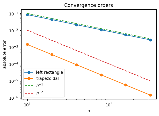
4. Monte Carlo Integration
4.1. Monte Carlo estimators
Integration equals expectationLet be a finite measure space with and consider .
First, notice that need not be a probability measure because may not be . We therefore normalize it by defining , and then define as a random point in distributed according to the normalized measure :
By the definition of expectation under this distribution, we then have:
If we multiply by , we obtain:
If we then set , take independent samples from the distribution of , and set
then we have
Thus, the Monte Carlo estimator is
By the LLN, we also know that as .
This is the Monte Carlo estimator of .
Furthermore, by linearity, we have
so we can conclude that the Monte Carlo estimator is unbiased.
For example, we can consider
Then we have
The exact value is
Why Monte Carlo is particularly good in high dimensions
Consider . Then:
and
- If we consider the deterministic rectangle rule with evaluations and an -Hölder function :
- If we use Monte Carlo, independently of :
Theorem: Strong Law of Large Numbers
Let be i.i.d., then:
Therefore, the Monte Carlo approximation is strongly consistent (i.e. it converges).
Theorem: Exact Root Mean Square Error
For i.i.d., we have:
ProofSince the estimator is unbiased, we can write:
By independence:
Therefore:
Thus, RMSE (reducing the error by a factor of 2 costs about 4 times as many samples).
4.2. Error analysis and practical integration
Estimating the unknown varianceConsider:
Two natural estimators are:
and the one using Bessel's correction:
Then:
Therefore:
Thus, is biased downward by , while is unbiased. However, note that both are consistent, so being unbiased does not imply a smaller RMSE.
Theorem: RMSE of the corrected sample variance
Assume are i.i.d. and consider:
Then, for :
Furthermore, for :
Corollary: RMSE of the biased sample varianceFor the biased sample variance defined above:
Regardless of :
Recall that is the fourth central moment, which measures how strongly observations can deviate from the mean, especially in the tails. It is used to calculate the kurtosis:
Recall also that, for a Gaussian distribution, . We define the excess kurtosis of a random variable as (which is 0 for a Gaussian distribution).
Confidence intervals | CLT only
Consider
The CLT gives:
Theorem: Asymptotically valid CLT confidence intervalsFor , which determine the left and right widths of the interval:
Equivalently, using the standard normal cumulative distribution function :
In other words, if
then the probability that the interval contains converges to .
For a symmetric interval, set . The coverage probability is then:
Using a "practical version" of this theorem, we can replace by
and obtain an asymptotically valid confidence interval defined as:
Practical Numerical Integration
Consider to be bounded and contained in:
We extend by zero outside :
Consider independent and uniformly distributed random variables on , i.e. are i.i.d. Since is uniform on :
Because is zero outside :
Therefore:
The Monte Carlo estimator is:
where is the volume of the enclosing box:
Example: High-dimensional financial integration: Portfolio Value at Risk (VaR)
In quantitative finance, evaluating risk metrics such as VaR for a portfolio of correlated assets requires computing high-dimensional expectations. We can use the approach proposed above by modelling asset returns as a multivariate Gaussian distribution (even if asset returns, especially stocks, are not normally distributed and have very fat tails!).
where is the vector of expected returns and is the covariance matrix.
Consider also as the portfolio weight vector, with . Given this, the total portfolio loss is defined as:
We can then define the Value at Risk, , as the -quantile of the loss distribution:
In Python, we can estimate the VaR for a -dimensional portfolio (in the snippet below: ) using Monte Carlo integration and tracking the convergence.
def run_portfolio_var_mc(d, N_list, alpha=0.95, rng=None):
if rng is None:
# Try to retrieve rng from globals, otherwise initialize a new one
global_vars = globals()
if 'rng' in global_vars:
rng = global_vars['rng']
else:
rng = np.random.default_rng(2026)
# Setup portfolio parameters (d=10 assets)
# weights vector
weights = np.ones(d) / d
# expected return (drift)
mu = np.linspace(0.01, 0.08, d)
# Generate a random positive-definite covariance matrix
A = rng.normal(size=(d, d))
# Covariance matrix \Sigma = 0.02 * AA^T + 0.05 I_d
# (the added identity improves stability and prevents \Sigma from being singular)
Sigma = np.dot(A, A.T) * 0.02 + np.eye(d) * 0.05
# Since this is Gaussian, we can calculate the analytical VaR for comparison
port_mu = np.dot(weights, mu)
port_vol = np.sqrt(np.dot(weights, np.dot(Sigma, weights)))
from scipy.stats import norm
# exact formulation
exact_var = -(port_mu + port_vol * norm.ppf(1 - alpha))
estimates = []
ci_lower = []
ci_upper = []
# we now proceed with estimation
for N in N_list:
# High-dimensional Gaussian sampling via Cholesky decomposition
L_mat = np.linalg.cholesky(Sigma)
Z = rng.normal(size=(N, d))
# R = \mu + Z L^T has approx. desired distribution
R = mu + np.dot(Z, L_mat.T)
# Portfolio losses
losses = -np.dot(R, weights)
# Estimate VaR (the empirical alpha-quantile)
# alpha-quantile of the simulated losses
est_var = np.percentile(losses, alpha * 100)
estimates.append(est_var)
# Bootstrap for quantile confidence intervals
bootstrap_vars = []
for _ in range(200):
boot_sample = rng.choice(losses, size=N, replace=True)
bootstrap_vars.append(np.percentile(boot_sample, alpha * 100))
# The interval is an approximate 95% bootstrap confidence interval for VaR.
ci_lower.append(np.percentile(bootstrap_vars, 2.5))
ci_upper.append(np.percentile(bootstrap_vars, 97.5))
return N_list, np.array(estimates), np.array(ci_lower), np.array(ci_upper), exact_var
# Fallback initialization in the script level if 'rng' is not defined globally
if 'rng' not in globals():
rng = np.random.default_rng(2026)
d = 10
N_list = np.logspace(2.5, 5.5, num=10, dtype=int)
Ns, estimates, ci_lower, ci_upper, exact_var = run_portfolio_var_mc(d, N_list, rng=rng)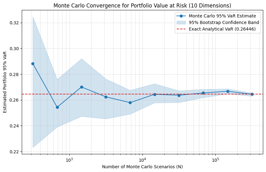
Monte Carlo: a short summary
The previous chapter can be summarized in 5 essential formulas:
Always remember the Monte Carlo rate , independently of the dimension of the problem.
Wiener Process from an Isonormal Gaussian Process
In this section, we want to characterize a one-dimensional Wiener process. To do that, we start with the isonormal Gaussian map.
Let and let be an orthonormal basis of . Assume that carries independent random variables .
For , define:
Then:
Therefore, we have:
The map is linear, and we also have:
Since every finite vector is jointly Gaussian, is an isonormal Gaussian process over .
We can now define the Wiener process by
The process is centered Gaussian, and
Therefore,
Furthermore, for two disjoint intervals and ,
Thus, the corresponding Gaussian increments are uncorrelated and therefore independent.
Sobolev–Slobodeckij path regularity
For and , we define:
By definition, Wiener process increments satisfy , with .
So, if we write , we have that:
and, by Tonelli, we have that:
This singularity at is integrable .
If we add that , we have that:
In particular, in one dimension, we have that when and .
If we fix any and choose large and then such that:
has a modification that satisfies
Numerical Picture of the Isonormal Construction
To visualize this, we can construct the Brownian motion numerically. First, we choose a real trigonometric orthonormal basis of :
We can then construct for every as
Recall that the space is
with inner product
In Python, we write:
def isonormal_brownian_trig(t, modes=200, rng=rng):
t = np.asarray(t)
W = rng.standard_normal() * t
for k in range(1, modes + 1):
xi_cos = rng.standard_normal()
xi_sin = rng.standard_normal()
int_cos = np.sqrt(2) * np.sin(2 * np.pi * k * t) / (2 * np.pi * k)
int_sin = np.sqrt(2) * (1 - np.cos(2 * np.pi * k * t)) / (2 * np.pi * k)
W += xi_cos * int_cos + xi_sin * int_sin
return W
5. Stochastic Integration and Itô Calculus
5.1. Stochastic processes and Brownian motion
Stochastic ProcessFix a complete probability space . We recall that a random variable is a mapping such that
We define a real-valued stochastic process as a family of real-valued random variables indexed by a non-empty set .
We often write instead of , .
Stochastic processes can be defined both in discrete time, where , and in continuous time, where . In the following notes, we consider for a finite .
There are three ways to interpret stochastic processes:
- for each time , as a random variable of the event
- for each event , as a sample path
- as a joint mapping of event and time
In continuous time, we usually require continuity properties for the sample paths and joint -measurability of .
Furthermore, two real-valued stochastic processes and on the same probability space are called:
- modifications if, for every , ;
- indistinguishable if there is an event with such that for every and .
Note that indistinguishability implies modification, but not conversely.
Definition: Filtration
A filtration on a probability space is a family of -algebras such that:
- for all ;
- whenever ("memory is perfect").
Intuition: -algebras represent information, while filtrations represent its flow over time.
A probability space equipped with a filtration is called a filtered probability space, denoted by .
Intuition: as time passes, contains everything known at time .
For example, for a Brownian motion , we often use:
Thus, contains the history of the Brownian motion up to time , but not its future.
Natural Filtration and AdaptednessThe natural filtration of a stochastic process is defined by:
The natural filtration describes the flow of information generated by observing the process over time.
Furthermore, a process is adapted to if is -measurable for every . Equivalently,
Therefore, adaptedness means that can be determined using only information available at time and cannot depend on the future.
For example, if contains the history of a Brownian motion up to time , then is adapted. However, is generally not -measurable because it depends on future randomness.
Usual Conditions for a FiltrationConsider or . A continuous-time filtration satisfies the usual conditions if it is:
- complete: if and , then ;
- right-continuous: for every before the terminal time.
Let
be the collection of null sets. The right-continuous completion is defined by
with when .
The completeness condition makes null events known at time . Right-continuity means that information available immediately after time contains nothing genuinely new compared with the information available at time .
Note that, in the context of stochastic integration, we usually work with filtrations satisfying the usual conditions.
Random Times and Stopping Times
Recall that or .
A random time is a random variable .
Generally speaking, a random time represents when a random event occurs.
Given a filtration , a random time is an -stopping time if
Intuition: at any fixed time , we can determine whether the stopping event has already occurred using only the information in .
Suppose that , that satisfies the usual conditions, and that is a real-valued, -adapted process with almost surely continuous paths. Then, for ,
is an -stopping time. Indeed, continuity of the paths gives
and right-continuity then implies .
Conditional Expectation
First, consider a real-valued random variable and a -algebra .
The conditional expectation is any random variable such that:
- is -measurable;
- ;
- for every ,
Let and let be a -algebra. Then exists and is unique up to almost-sure equality.
Furthermore, conditional expectation defines a positive, continuous, linear operator.
Properties of Conditional ExpectationsAssume that all random variables are integrable and that and are -algebras.
-
If is -measurable, then .
-
If is -measurable, then almost surely.
-
If and are independent, then almost surely.
-
If , then
almost surely (the tower property).
-
For a convex function such that the expectations exist,
almost surely (conditional Jensen's inequality).
-
If is an increasing sequence of nonnegative random variables converging to , then conditional monotone convergence gives
-
If almost surely and almost surely for an integrable random variable , then conditional dominated convergence gives
-
If almost surely for an integrable random variable , conditional Fatou's lemma gives
Martingales
A stochastic process is an -martingale if:
- is -adapted;
- for every ;
- almost surely whenever .
A family is uniformly integrable if
If and , then is a uniformly integrable martingale.
Brownian Motion
Consider or . A standard one-dimensional Brownian motion (Wiener process) is a continuous stochastic process such that:
- almost surely;
- the sample paths are almost surely continuous;
- for every , the increments are independent;
- for ,
An -dimensional Brownian motion is a column vector whose components are independent standard one-dimensional Brownian motions.
Brownian Motion Relative to a Filtration
We often want a stochastic process to be a Brownian motion with respect to the flow of information modeled by a filtration.
Given a filtration , a process is called an -Brownian motion if:
- is -adapted;
- is a Brownian motion;
- for every , the future-increment process is independent of .
Every Brownian motion is a -Brownian motion, where is the right-continuous completion of its natural filtration.
Furthermore, the map is -measurable.
-Variation of Brownian Motion
For and , define the -variation along the dyadic partitions by:
when the limit exists. The -variation is called the total variation (it adds up all the absolute increments and measures the "total distance" traveled by the path), and the -variation is called the quadratic variation (it adds up the squares of the increments and, for Brownian motion, captures the accumulated randomness).
For larger , small increments become much smaller after taking the power, so the sum is less sensitive to fine-scale fluctuations.
For Brownian motion, almost surely:
Then, for any , we have
Martingales for Brownian Motions
Let be an -Brownian motion. Then:
- is a square-integrable -martingale.
- The process is an -martingale.
- For any , the process is an -martingale.
5.2. Itô integration and calculus
Stochastic Itô Integral of Simple ProcessesLet for some . We fix the same probability space supporting an -Brownian motion .
A stochastic process is a simple process if there exist times and bounded -measurable random variables such that:
The stochastic integral of a simple process is then defined as:
where .
Intuition (gains/losses of a self-financing trading strategy): in finance, we assume the stock moves as Brownian motion. At time , we buy shares at price and at time we sell at price , so the integral between and is just the P&L in this trade. Note that has to be -measurable in order to get the number of shares to buy.
Then, Itô's isometry holds for all :
Intuition: Itô's isometry states that the expected squared size of the stochastic integral equals the expected accumulated squared size of the integrand.
Then, the process is a square-integrable martingale.
Then, again, for simple processes and and , we have the very nice linearity property:
The continuity property also holds, since the sample paths are continuous.
Simple Processes: The Martingale Property
Let , which is adapted by definition and square-integrable by Itô's isometry.
We fix and refine the partition without changing or , so that and . Then we have:
For , we have that .
The tower property, the independence of the Brownian increments, and their zero mean () give:
The first equality holds since , and the second equality follows because is independent of .
If we sum over , we obtain:
Stochastic Itô Integral of Square-Integrable Processes Definition: Predictable -algebra
The predictable -algebra on is the -algebra generated by all left-continuous and -adapted processes .
Note that the predictable -algebra can also be defined as the -algebra generated by all simple processes .
For a predictable process , we define the norm as:
Note that since is predictable, it is also progressively measurable, i.e. is -measurable (intuition: up to time , the whole path of is determined by information known at ).
For each , there is a sequence of simple processes such that
Intuition: simple predictable processes are dense in the space of square-integrable predictable processes. Their stochastic integrals therefore approximate the stochastic integrals of those processes in , by Itô's isometry.
We now spend some time showing that every square-integrable predictable process can be approximated in by simple processes.
We first truncate the square-integrable process by defining:
(This bounds in the interval .) Since pointwise and , dominated convergence gives:
We then extend for and define the moving average over the recent past (bounded by , continuous, and adapted in ):
Lebesgue differentiation and dominated convergence give in as .
We then discretize at left endpoints. For , we set:
For fixed and , uniform continuity and dominated convergence give in as . Therefore, a diagonal sequence gives in .
Then, is a Cauchy sequence, i.e. for :
By Itô's isometry, for every :
Therefore, is a Cauchy sequence in .
Since is complete, there exists a random variable such that
Therefore, for , we define the stochastic integral by:
where is a sequence of simple processes satisfying:
Again, Itô's isometry holds:
The process is a square-integrable martingale; as stated above, linearity and continuity also hold.
Doob's Maximal Inequality Theorem
If is a right-continuous, square-integrable -martingale, then:
In particular, for a simple process, Doob's inequality and Itô's isometry give:
Furthermore,
Associativity of Stochastic Integrals
For a predictable process and , we have:
In general, for predictable processes and such that :
Furthermore, if is a simple process, then:
Intuition: the stochastic integral with respect to the martingale accumulates the values of against the increments of that martingale.
Stochastic Itô Integrals of Predictable Processes
Finally, we can define the stochastic integral for predictable processes satisfying
using the localization technique.
For each , define the stopping time:
Intuition: represents the size, or energy, of . The stopping time is the first time this size exceeds .
The sequence is a localizing sequence of -stopping times.
We define the stopped integrand by
Then is square-integrable, and
is well-defined. The family is consistent, meaning that for :
Therefore, for :
However, note that, since we use the localization technique, the integral is no longer necessarily an -martingale, but only an -local martingale.
(Recall that a stochastic process has a property locally if there exists a localizing sequence such that the stopped process has property .)
Luckily, we still have the linearity property for two predictable processes and :
In particular, the mapping
is a continuous linear operator, where the metric is defined by
Burkholder–Davis–Gundy Inequalities
For , define . Then there exists such that:
- BDG 1: terminal-time estimate
- BDG 2: maximal estimate
Furthermore, for , Minkowski's inequality gives:
Quadratic Variation
For , the quadratic variation satisfies:
For the dyadic partition, define
Itô Calculus
Itô processes are given by:
This is shorthand for the integral equation, for :
Here, and are predictable processes such that
Differentials are a tool for computation using the following rules:
- .
- .
- .
Therefore,
Here, denotes the quadratic variation of up to time , defined as:
Recall also that, for a Brownian motion, , usually written as .
Itô's FormulaGiven a function and an Itô process
the process is also an Itô process satisfying:
For example, if , then , so and . According to Itô's formula:
Multidimensional Itô Processes
Suppose that is an -dimensional Brownian motion. Consider the -dimensional Itô process given by:
Here, and are predictable stochastic processes such that the integrals are well-defined.
Moreover, the Itô multiplication rules are:
- ;
- ;
- , where if and otherwise.
For a function , define . The multidimensional Itô formula is:
Integration by Parts
Suppose we have an -dimensional Brownian motion and the pair of Itô processes:
Then the product is still an Itô process satisfying:
Numerical Illustrations of Stochastic Integration
In the following section, we spend some time showing "numerically" and "visually" what we've done so far by showing some processes and examples.
Firstly, we just defined Brownian Motion by continuity, independent increments and:
which can be simulated with the following script of code.
rng = np.random.default_rng(20261015)
def brownian(T=1.0, N=5000, dim=1, rng=rng):
dt = T/N
dW = np.sqrt(dt)*rng.standard_normal((N, dim))
W = np.vstack([np.zeros((1, dim)), np.cumsum(dW, axis=0)])
t = np.linspace(0.0, T, N+1)
return t, W.squeeze()
t, W = brownian(T=2.0, N=10_000, rng=rng)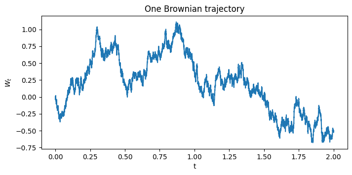
We can now further define a basic stopping time as:
that, for our Brownian motion, translates to
that brings us to the following:
a = 1.0
idx = np.flatnonzero(np.abs(W) >= a)
i_tau = idx[0] if len(idx) else len(W)-1
plt.scatter([t[i_tau]], [W[i_tau]])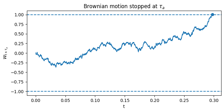
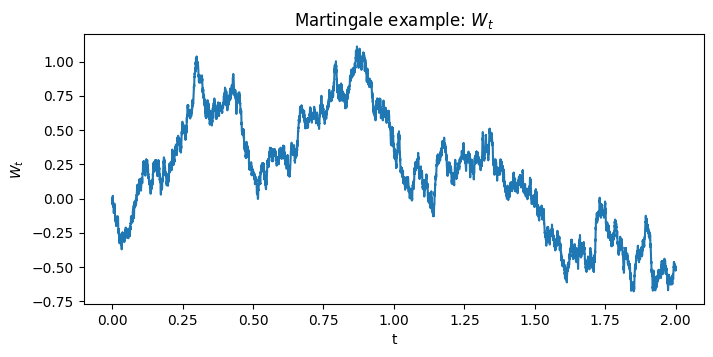
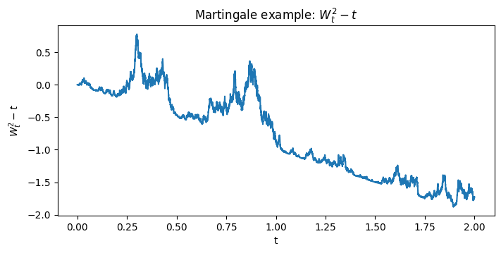
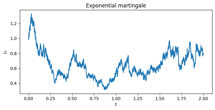
We now show three different Brownian Martingales (, , ), but note that from a single trajectory we cannot prove the martingale property; we can only see its typical path shape.
We now spend some time illustrating a simple predictable process and its Itô Integral. We define it by:
Then the integral can be built exactly from the increments as follows:
T = 1.0
N = 2000
t2, W2 = brownian(T=T, N=N, rng=rng)
dW2 = np.diff(W2)
# Use blocks of 40 simulation steps as the simple-process partition.
block = 40
K = np.zeros(N)
for j in range(0, N, block):
K[j:min(j+block, N)] = 1.0 if W2[j] >= 0 else -1.0
I = np.concatenate([[0.0], np.cumsum(K*dW2)])
plt.plot(t2, I)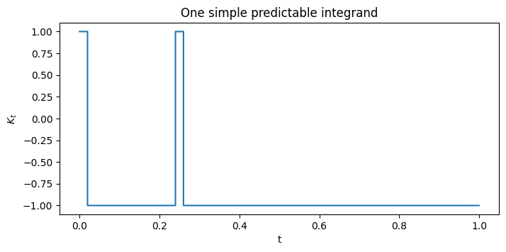
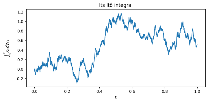
Furthermore, if we consider , Itô's formula gives the following exact identity:
where the first identity comes from Itô’s formula applied to with , and the second one from integrating from to and using .
So the stochastic integral can be approximated by left-point sums:
dW2 = np.diff(W2)
I_left = np.concatenate([[0.0], np.cumsum(W2[:-1]*dW2)])
I_exact = 0.5*(W2**2 - t2)
plt.plot(t2, I_left, label="left-point Itô sum")
plt.plot(t2, I_exact, "--", label=r"Exact formula")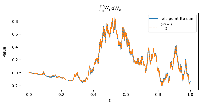
We now consider the quadratic variation of a stochastic integral that, again for , is defined as:
dI = np.diff(I_left)
qvI = np.concatenate([[0.0], np.cumsum(dI**2)])
dt = T/N
rhs_qv = np.concatenate([[0.0], np.cumsum(W2[:-1]**2 * dt)])
plt.plot(t2, qvI, label="discrete quadratic variation")
plt.plot(t2, rhs_qv, "--", label=r"integral")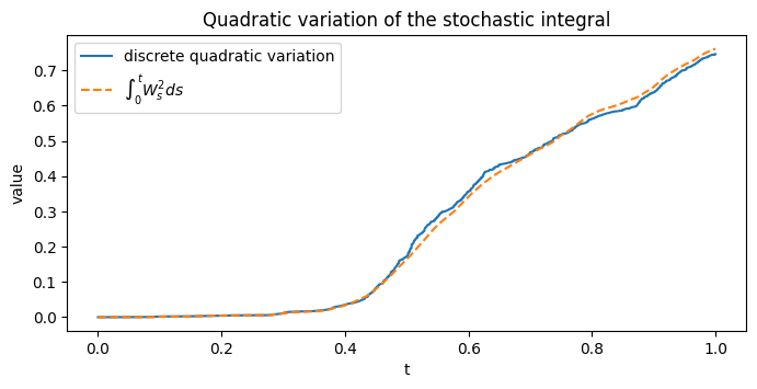
6. Stochastic Ordinary Differential Equations
6.1. SDE formulation and well-posedness
Let for some , consider , and let be the state space (intuition: is the set of possible values of the state process ; it is a measurable subset of ).
We fix a filtered probability space satisfying the usual conditions and supporting an -dimensional -Brownian motion .
We then consider Borel-measurable functions
called the drift coefficient and diffusion coefficient, respectively. We also consider an -valued, -measurable random variable .
Intuition: is the drift, i.e. the predictable and deterministic tendency of the process. is the diffusion, i.e. the random fluctuation of the process. Since , its typical size is .
We can also call the noise sensitivity, which determines how strongly each Brownian-motion component affects each coordinate of , and the initial state.
An equation of the form:
is called a stochastic differential equation (SDE).
An -valued process is a solution process of the previous SDE on the given filtered space if:
- is -adapted and has continuous sample paths.
- The following integrability condition holds:
- For every , -almost surely:
We also recall that is the Euclidean norm, and
Note also that the differential notation can be translated into the integral equation. For the th component, :
Note that and are predictable. In this case, a solution is an -valued Itô process with drift and diffusion coefficient .
We now consider , so is an -dimensional -Brownian motion whose components are real-valued.
For a random vector or matrix , we can then set, using the Euclidean norm on and the Hilbert–Schmidt norm on :
Recall that the Hilbert–Schmidt norm measures the size of a matrix by treating all its entries as orthogonal components (i.e. calculating the norm as if every entry were an independent coordinate in a Euclidean vector: a general matrix is flattened into a vector, and we take the usual Euclidean length, so cross-terms do not appear and we simply sum the squares of the entries).
For a matrix , we formally write:
In the case of , we have:
This is also called the Frobenius norm for finite matrices ().
Given these prerequisites, we can say that the coefficients and are globally Lipschitz if, for some ,
(Intuition: changing the input from to changes the coefficients by at most a constant multiple of .)
Note that Lipschitz coefficients imply linear growth (by the triangle inequality) with :
Intuition: the coefficients may grow as grows, but not faster than linearly, and this prevents the SDE solution from exploding in finite time.
Theorem: Existence and uniqueness of solutions
Let , let be -measurable with , and let and be globally Lipschitz coefficients. Then:
- On a given filtered probability space, the usual SDE (defined above) has a solution that is unique up to indistinguishability.
- This solution has uniformly bounded -th moments:
- There is a constant such that
In particular, for every .
Intuition: uniqueness up to indistinguishability means that, once the initial state and entire random input are set, the SDE determines a unique trajectory. Note also that this is stronger than saying for every , because indistinguishability implies equality of the entire paths simultaneously.
Locally Lipschitz Coefficients
We now allow an open state space and consider
The coefficients and are locally Lipschitz if, for every compact set , there is a constant such that, for all ,
Note that, in this case, the constant may depend on , so different regions can have different Lipschitz constants. Of course, every globally Lipschitz function is also locally Lipschitz, but not vice versa.
For example, the function is locally Lipschitz on because its derivative is bounded on every compact interval. However, it is not globally Lipschitz, since the ratio
can become arbitrarily large.
We also recall that a set is open if every point has a "small neighborhood" contained in , i.e. there is "enough space" to move slightly in any direction while remaining in . For example, is an open set.
On the other hand, a set is compact if it is closed and bounded.
Theorem: Uniqueness for locally Lipschitz coefficients (pathwise uniqueness)
Let be open, let and be locally Lipschitz, and let be -measurable. Consider two -valued solution processes and of the usual SDE defined above, on the same filtered probability space, with the same Brownian motion and the same initial condition .
Then and are indistinguishable, that is:
In this case, no additional moment assumptions on are required. This is a uniqueness result; existence on is assumed.
Theorem: Existence of maximal solutions
Let and let be open, with and locally Lipschitz.
Then there is a local solution consisting of a stopping time and a continuous, adapted, -valued process on such that:
Intuition: we can consider as the stopping time called the explosion time, i.e. the SDE behaves normally until . After , something becomes "too large" or the process reaches the boundary of the state space, so the solution cannot continue while remaining in .
We also have the following condition (uniqueness and maximality): any other local solution with the same Brownian motion and initial state satisfies and for all .
Intuition: this means that exists at least as long as any other solution is defined, and all solutions agree while both are defined. In this case, we call the maximal solution.
Furthermore, on , eventually leaves every compact subset of as . For , this means that as .
Example: Brownian Motion
We now proceed with a very illustrative example. In particular, we assume that the initial value is deterministic and let , , , and .
We then set and , so the SDE becomes:
Note that in this case both coefficients are globally Lipschitz, since we have:
The bound is valid for all , and the coefficients satisfy the linear growth condition.
Therefore, the theorem gives a solution that is unique up to indistinguishability.
We now spend some time solving the equation.
Firstly, we see that the noise and the drift are proportional to , so dividing formally by suggests:
We can then apply a similar transformation using Itô's correction, with , since and .
Therefore, applying Itô's formula gives:
We now substitute and , since , , and the cross-term in Itô's formula. We obtain:
Integrating this equation from 0 to and using gives:
The factor is called the Itô correction.
Moreover, we can calculate the first moment. Because , we have:
Therefore, for deterministic :
Similarly, we can calculate the second moment using
and we get:
From the second moment, for , we have:
In Python, we can replicate numerically
alpha, beta, xi = 0.05, 0.20, 100.0
W, dW = brownian_path(1)
W = W[:, 0]
# exact solution
X_gbm = xi * np.exp((alpha - beta**2 / 2) * tgrid + beta * W)
mean = xi * np.exp(alpha * tgrid)
ax.plot(tgrid, X_gbm, lw=0.8, label=r'one trajectory')
ax.plot(tgrid, mean, 'k--', lw=1.2, label=r'deterministic mean')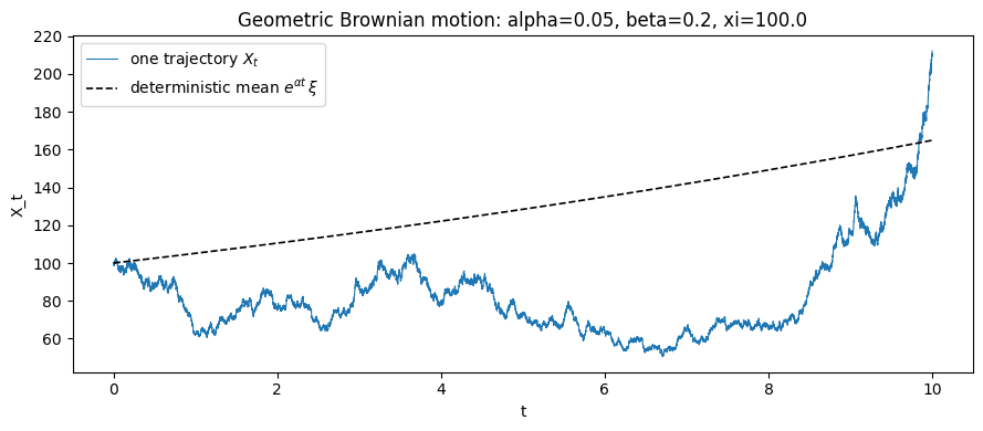
6.2. Examples and numerical illustrations
Examples: the Black-Scholes modelWe now consider another very famous example! Let , , , , , and . The coefficient functions are:
The corresponding system of SDEs is:
Again, the coefficients extend to globally Lipschitz functions on , and the unique solution is given by:
Here, notice that represents a bank account with interest rate , and represents a risky asset with expected return and volatility .
In Python, we can replicate it numerically with the following code.
r, alpha_bs, beta_bs = 0.02, 0.06, 0.25
xi1, xi2 = 100.0, 100.0
X1 = xi1 * np.exp(r * tgrid) # deterministic
X2 = xi2 * np.exp((alpha_bs - beta_bs**2 / 2) * tgrid + beta_bs * W)
ax.plot(tgrid, X1, lw=1.2, label=r'bank account ')
ax.plot(tgrid, X2, lw=0.8, label=r'risky asset ')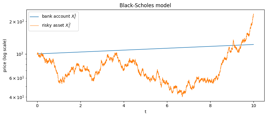
Example: the Cox–Ingersoll–Ross process
Consider , , , , and . The Cox–Ingersoll–Ross (CIR) process solves:
Here, and . For , the diffusion coefficient is locally Lipschitz but not globally Lipschitz near zero. Furthermore, if , there is a unique solution that remains in .
Note that the term represents the mean reversion: if the quantity is negative, the process is pushed downward, and vice versa. The equilibrium level is (the deterministic equation converges to ).
Note that this process is used to model instantaneous interest rates (, which are nonnegative and mean-reverting quantities) or the square of the volatility (variance) of asset prices, as in the Heston model. It captures nonnegativity, mean reversion, larger fluctuations when variance is high, and volatility clustering, i.e. large price movements tend to occur near other large price movements and vice versa.
In Python, we do the following.
alpha_cir, delta_cir, beta_cir = 0.5, 0.05, 0.25
xi_cir = 0.04
assert 2 * delta_cir >= beta_cir**2, "Feller condition 2*delta >= beta^2 violated"
mu = lambda x: delta_cir - alpha_cir * x
sig = lambda x: beta_cir * np.sqrt(max(x, 0.0))
X_cir = euler_maruyama(xi_cir, mu, sig, W, dim=1)[:, 0]
ax.plot(tgrid, X_cir, lw=0.8)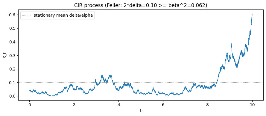
Example: the Heston stochastic volatility model
Let , , , and .
For , define
Then is a Brownian motion, and it is independent of if and only if . Its correlation with is , while its correlation with is .
The Heston model is the system:
Here, models the asset price and is its instantaneous variance; the second equation is a CIR SDE as written above. Note also that if , there is a unique positive solution. (However, the coefficients are not globally Lipschitz.)
Therefore, we can write the model in the more familiar form:
where is the asset price, is the instantaneous variance, is the instantaneous volatility, is the expected return, is the speed at which the variance returns to its long-run level , and controls the randomness of the variance.
In Python, we do the following:
al_h, alh, delh, beth = 0.05, 1.0, 0.08, 0.25 # asset drift; variance mean-reversion params
rho = 0.7
x0 = np.array([100.0, 0.04])
assert 2 * delh >= beth**2, "Feller condition for the variance process violated"
Wh, _ = brownian_path(2) # (W^1, W^2)
WhW = np.sqrt(1 - rho**2) * Wh[:, 0] + rho * Wh[:, 1] # correlated driver
X_h = np.empty((N + 1, 2)); X_h[0] = x0
for k in range(N):
dW1 = Wh[k+1, 0] - Wh[k, 0]
dWh = WhW[k+1] - WhW[k]
v = max(X_h[k, 1], 0.0)
X_h[k+1, 0] = X_h[k, 0] + al_h * X_h[k, 0] * dt + X_h[k, 0] * np.sqrt(v) * dW1
X_h[k+1, 1] = X_h[k, 1] + (delh - alh * X_h[k, 1]) * dt + beth * np.sqrt(v) * dWh
X_h[k+1, 1] = max(X_h[k+1, 1], 1e-12)
ax1.plot(tgrid, X_h[:, 0], lw=0.8, color='tab:blue')
ax2.plot(tgrid, X_h[:, 1], lw=0.8, color='tab:red')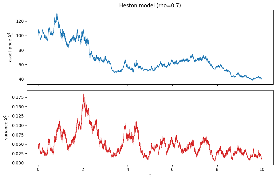
7. Tractability
7.1. Explicit solutions and generators
We now try to understand what we can calculate from a stochastic differential equation without relying entirely on simulated paths (i.e., when computing simulated paths is costly).
In particular, we will take a deep dive into three possible types of tractability:
- explicit solution, where a formula gives exact updates on a time grid
- explicit transition law, where we can derive the conditional distribution at a later time, either for direct sampling or integration
- tractable Fourier–Laplace transform, where we can derive a formula or an ODE system for a transform, and then its inversion can give quantities.
Note that these types may overlap: one model may have more than one type of tractability.
Explicit Solution | Black–Scholes and Geometric Brownian Motion
We can start by considering the Black–Scholes model as before, with and .
First, we can solve the SDE explicitly by applying Itô's formula to . This gives:
Since and , we can write:
If we now integrate from to and use and , we get:
From the same model, we can calculate the marginal law and moments.
Indeed, since and , the marginal law is:
Therefore, is lognormally distributed.
Then, for all , the Gaussian moment-generating formula, , gives:
In the particular case , we can calculate the expected value as .
We can now compare the exact transition and the Euler preview. In particular, we know that:
While Euler uses:
Recall that the Euler preview is an approximate way to step the price forward (if we do not know the exact solution). If we start at price at time , we freeze the drift and volatility for one small interval . The Brownian-motion increment during that interval is (whereas the Black–Scholes update uses the exponential formula).
Therefore, we can simply exponentiate the exact increments in the log-price for the exact formula and then use Euler, by freezing coefficients at each step, to compare them.
T,N=1.0,80 #Change T to broadcast changes to discretization vs exact method: the bigger T gets, the higher the discrepancy between the 2 methods. Try e.g. T=50.
dt=T/N
s0,mu,sig=100.0,0.08,0.25
dW=np.sqrt(dt)*rng.standard_normal(N)
t=np.linspace(0,T,N+1)
Sx=np.empty(N+1); Se=np.empty(N+1)
Sx[0]=Se[0]=s0
for n in range(N):
Sx[n+1]=Sx[n]*np.exp((mu-.5*sig**2)*dt+sig*dW[n])
Se[n+1]=Se[n]+mu*Se[n]*dt+sig*Se[n]*dW[n]
plt.figure(figsize=(8,3.5)); plt.plot(t,Sx,label='exact'); plt.plot(t,Se,'--',label='Euler preview')
plt.xlabel('t'); plt.ylabel('S'); plt.title('Black–Scholes'); plt.legend(); plt.show()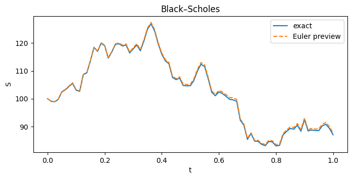
Explicit Solution | Multivariate Black–Scholes
Similarly, we can consider an -dimensional Brownian motion and an -dimensional Black–Scholes model, with (how the assets move together). The diagonal entries are , the variance rates of the individual assets:
In this case, by applying Itô's formula to each and using , we obtain:
So, this is still explicit-solution tractability: the assets' exact values can be calculated from the initial prices and Brownian motion, without using an Euler approximation.
Again, if we want to compute the joint law, we can integrate the log-price equations:
Since is Gaussian with covariance , we have:
Therefore, the asset prices are jointly lognormally distributed.
Again, we can perform a numerical check and compare the asset paths coordinate by coordinate using the exact formula and Euler approximation.
T,N=1.0,100; dt=T/N; d=3
S0=np.array([100.,80.,120.]); mu=np.array([.06,.03,.08])
Sigma=np.array([[.20,0,0],[.10,.18,0],[.06,.04,.22]])
a=Sigma@Sigma.T
dW=np.sqrt(dt)*rng.standard_normal((N,d)); t=np.linspace(0,T,N+1)
Sx=np.empty((N+1,d)); Se=np.empty((N+1,d)); Sx[0]=Se[0]=S0
for n in range(N):
shock=Sigma@dW[n]
Sx[n+1]=Sx[n]*np.exp((mu-.5*np.diag(a))*dt+shock)
Se[n+1]=Se[n]+mu*Se[n]*dt+Se[n]*shock
plt.figure(figsize=(8,4))
for i in range(d):
plt.plot(t,Sx[:,i],label=f'asset {i+1} exact')
plt.plot(t,Se[:,i],'--',alpha=.65)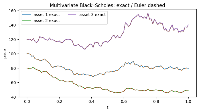
Explicit Solution | Multivariate Ornstein–Uhlenbeck Process
We can consider a vector-valued process such that
Here, is the long-run mean, controls how quickly the process moves back toward its mean (since is a matrix, the coordinates can influence one another), and controls the random fluctuations and their correlations.
To obtain the explicit solution, subtract and write the drift as :
Now multiply by the integrating factor and use the product rule. Since is deterministic and differentiable:
Substituting , the drift terms cancel:
Integrating from to and using , we obtain:
The stochastic integral is Gaussian, so has a Gaussian distribution:
More generally, given the current state , the state after an interval is:
So we can sample the next state directly from this Gaussian distribution. Again, this is explicit transition-law tractability (i.e., no small Euler steps are needed to get the exact distribution at the next grid point).
Furthermore, note that if all the eigenvalues of have positive real parts, then decays as grows. The covariance therefore converges to , which solves:
Therefore, is the invariant distribution (if the process starts with this distribution, it keeps it over time).
Again, we perform a numerical comparison between the exact Gaussian transition, sampled using a Cholesky factor of its covariance, and the usual Euler discretization (using the same normal draws).
T,N=5.0,250; dt=T/N
K=np.array([[1.4,-.35],[.20,.90]])
theta=np.array([1.0,-.5]); Sigma=np.array([[.65,.10],[0,.45]])
Q=Sigma@Sigma.T; x0=np.array([3.0,1.5])
Cinf=solve_continuous_lyapunov(K,Q)
E=expm(-K*dt); Cdt=Cinf-E@Cinf@E.T; Cdt=.5*(Cdt+Cdt.T)
L=np.linalg.cholesky(Cdt+1e-14*np.eye(2))
Z=rng.standard_normal((N,2))
Xx=np.empty((N+1,2)); Xe=np.empty((N+1,2)); Xx[0]=Xe[0]=x0
for n in range(N):
Xx[n+1]=theta+E@(Xx[n]-theta)+L@Z[n]
Xe[n+1]=Xe[n]+K@(theta-Xe[n])*dt+Sigma@(np.sqrt(dt)*Z[n])
t=np.linspace(0,T,N+1)
plt.figure(figsize=(8,4))
for i in range(2):
plt.plot(t,Xx[:,i],label=f'coord {i+1} exact')
plt.plot(t,Xe[:,i],'--',alpha=.7)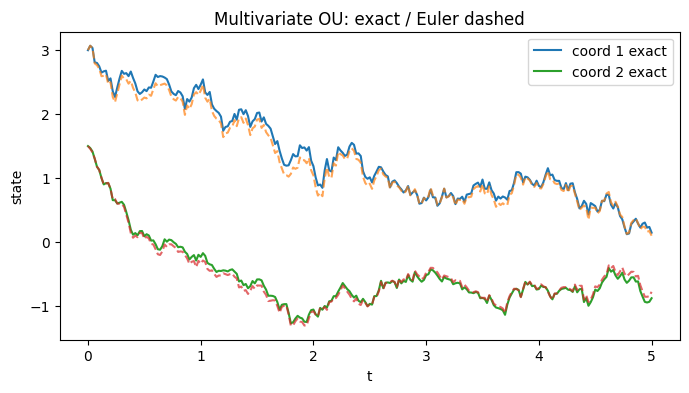
Generator of a General Diffusion
The starting idea is that the generator describes how the expected value of a function of a diffusion changes over an infinitesimally small short time.
Firstly, consider a stochastic differential equation of the form:
where is the state of the system, is an -dimensional Brownian motion, the drift, and the diffusion matrix.
The SDE says that, for a small time interval , we have
where is the local average displacement and is the random displacement. Furthermore, since Brownian motion increments are , we have that
Therefore, if we start at , we have that
where is the instantaneous covariance of the state increments.
Consider now a sufficiently smooth function and think of as an "observable" of the system (its positions, squared position, payoff etc...).
The generator is defined, if the limits exist, as:
or, equivalently,
Intuition: is the instantaneous rate of change of the expected observable starting at . Note that the expectation comes first: indeed, the generator does NOT describe any derivative of a Brownian path (also because they are not generally differentiable!)
In the case of the diffusion above the generator is:
where is the gradient, is the Hessian matrix with all the second derivatives and is the trace (sum of diagonal entries). Note that in the formula represents the effect of the drift, the remaining part the effect of randomness.
Derivation of the generatorSuppose we have . Over a short interval, we can write:
We then expand with Taylor around and take expectations to get:
We now notice that so, to first order in , we also have , so we can write:
and, by dividing by and taking the limit:
Note that we have a second derivative because a Brownian increment is typically of size , so its square is of size . Therefore, as , the second-order Taylor term contributes at the same order as the drift term and so we have the second derivatives.
Furthermore, even if the random displacement has zero mean, its variance can change the expected value of a curved function. For example, take and add zero-mean noise. In this example, the expected square increases.
Example: Dynkin's formula
We now prove Dynkin's formula by calculating .
For a sufficiently smooth , we can apply the multidimensional Itô's formula:
We then substitute so we can have:
and immediately notice that what is in the brackets is exactly , so we can write:
If we now integrate from to (with , ):
If , then .
If we assume sufficient integrability, the stochastic integral is a true martingale with zero expectation, so we have:
that is precisely Dynkin's formula.
Intuition: the generator returns the instantaneous expected change, while Dynkin’s formula adds that change up over time, so the expected value at is the initial value plus the accumulated expected value of the generator.
Furthermore, we've nicely seen that for a time-homogeneous Markov diffusion, if is sufficiently smooth and belongs to the generator’s domain, the coefficient of in Itô’s formula is .
Basic Properties of the Generator
- is linear
- If has a local maximum at an interior point , then (positive maximum principle)
- for we have
The idea behind the first point is that, if we take the constant function , the gradient and the Hessian are zero (, ), therefore (intuition: a constant never changes and its instantaneous expected change must be zero)
Furthermore, if we consider smooth functions and constants , since differentiation is linear we have:
So the generator is
Furthermore, we can interpret as the transition operator. In this context, takes observable and returns a new function of the starting point , so is what we measure, is its expected value at .
Lastly, the intuition behind the last property is that the rate of change of the expected observable is the expected value of its generator.
Example: generator as a short-time derivative
Consider now the 1D Ornstein–Uhlenbeck process, that is:
where, again, is the long-run mean, controls the mean reversion and the noise. In this case, the drift is , so if the overall drift is negative and the process is pulled down.
The one-dimensional generator for is:
where the first term represents the mean-reverting drift and the noise (note that this is positive even if the noise has zero mean, since it indeed increases the expected square with its variance).
Affine Transforms
In this section, we understand how to calculate useful information about the future of an SDE without simulating thousands of paths. Indeed, often the distribution of an SDE is difficult to write down explicitly, but we may be able to calculate the transform of that distribution.
In particular, a transform takes an expectation of a convenient function of the random variable, for example, the Laplace transform is defined as , the characteristic function as , so we clearly see that they summarize the distribution.
Once we know the transform, we can use it to calculate the moments or, with Fourier inversions for example, prices of financial derivatives.
In particular, we are interested in the special feature of an affine process, i.e. that its transform has an exponent that is affine in the initial state, in one dimension this means:
where is the starting value (), determines which transform we calculate and , depend on time and .
The intuition is that we can find and by solving ordinary differential equations, rather than solving a full partial differential equation or simulating paths.
CIR Process
We now consider a CIR process defined by:
and we derive its generator by applying Itô's formula:
where we can substitute and (remember that Brownian motion increments have variance , so their squares accumulate at order ) so we have:
and we remember that the generator is the coefficient of , so we have:
Furthermore, since , it is convenient to define the Laplace Transform as
To calculate , we proceed as follows. We want to find an exponential-affine expression , called an ansatz, that is equal to the Laplace transform and has the following form:
The backward equation tells us to require
Furthermore, since , the initial condition must hold, i.e.
that, if we write in the ansatz form, gives and .
We now compute the derivatives of holding fixed (a dot denotes a derivative with respect to ) and with respect to holding fixed.
We now substitute these derivatives in the generator function that, as stated before, has the form:
If we set (from the backward equation) and we divide by :
and, since this has to hold for every , we must have:
and the coefficients of must match:
Note that the equation for is called a Riccati equation because it contains the quadratic term . However... we're not done yet.
For , we put , then we can write:
so we can solve the linear equation and take the reciprocal:
Finally, we integrate and we obtain:
Therefore, we found a function that satisfies the backward equation, but this is only the starting point: we indeed have to connect it to the expectation.
So we fix a future time and we move "forward in the process, backward in time"
Intuition: as increases, moves forward on its random path, while the time argument decreases to .
Since depends both on time and , we can apply Itô's formula and we get:
But satisfies the backward equation , so the coefficients cancel out and we have:
and we immediately notice that is a local martingale since it has no remaining drift.
For , we have, according to the above formulas, and, since , we have:
So here every stopped process is bounded in and we can use dominated convergence as the stopping times move out to infinity (so we can consider processes and not stopped processes) and so the martingale property of the stopped processes passes to directly, so we have,
Therefore, is a true martingale and, if we take expectations on both sides, we have , which means that the expected value is constant.
Coming back to the beginning, its expectations must be the same also at the endpoints, so we must have that, if we substitute, gives:
Heston Model
We now consider and, under a pricing measure, we define on the state space :
The Heston Model describes a stock whose volatility changes randomly over time, where is the log stock price, is the instantaneous variance ( is volatility).
In the model, the stock's log return is , where is the risk-free rate, the dividend yield and comes from taking the log. Furthermore, variance has a long-run level to which it comes back at a speed and controls how "randomly" variance fluctuates. Brownian motions (for the stock) and (for the variance) have correlation .
Furthermore, we consider the Fourier transform in and the Laplace transform in that summarize the joint distribution of log price and variance.
In particular, is the Fourier part ( denotes the distribution of the log price) and is the Laplace part ( denotes the distribution of the variance). The expectation then averages their product over all outcomes, capturing how and move together.
As we've done before, we will write the generator, propose an exponential-affine expression, use the backward equation and obtain equations for , .
For the Fourier–Laplace transform, we consider and, for the characteristic function of , we consider , so we can write:
and we propose the following exponential-affine form where , depend on and (but we suppress this to keep the notation friendly!)
Intuition: as before, we do not directly calculate the expectation over all possible random paths, but we look for two deterministic functions , that characterize the expectation.
We start with the initial conditions. At , , , so we have:
The ansatz at is , so we need:
We now derive the generator considering a sufficiently smooth function and applying the 2-dimensional Itô's formula:
In this expression we have:
- for the diffusion part of , we have that
- for the diffusion part of , we have that .
- for the cross-variation we use the correlation defined above:
We now substitute these into Itô's formula and we take the coefficient of , so we end up with the Heston Generator that describes the expected change of a function of the state.
In the formula, the first two terms come directly from the drifts of , . , come from their random fluctuations and from their correlation.
As before, we now apply the backward equation, so we require where is time from the initial state.
We now calculate each derivative for :
Now we start from the generator formula, defined above, we apply the derivatives, we expand each term, separate those with and without and finally combine the coefficients for , so we have:
We now set and, cancelling , we have:
and, since this must hold for every starting variance , we can use the initial conditions to derive:
However, so far we have shown that the candidate satisfies the backward equation and the initial conditions. We now connect it to the expectations using the "forward in process, backward in time" approach (same for the CIR process above).
We indeed fix and we define:
As shown before, is a true martingale and we have , but we also have:
Therefore, for a real and , this is the bounded Fourier–Laplace transform.
Heston Model: a numerical comparison
We now spend some time checking the Heston transform derived above by comparing two solutions:
- the Riccati ODE by numerically solving the equations for ,
- the Euler Monte Carlo by simulating many approximate Heston paths and averaging the transform over them
In particular, both approaches estimate:
# Heston joint Fourier–Laplace transform:
# Riccati ODE versus empirical Euler transform
import numpy as np
from scipy.integrate import solve_ivp
rng = np.random.default_rng(20261015)
# #risk free, dividdent yield
r, q = 0.02, 0.0
# long run mean, speed reversion, volatility of variance, correlation
kappa_h, theta_h, xi_h, rho = 1.8, 0.04, 0.45, -0.7
# starting values
x0_h, v0_h = np.log(100.0), 0.04
T_h = 1.0
eta_laplace = 2.0For the Riccati approach, we use the formula derived before. Note that, the small tolerances request a precise ODE solution. This is still a numerical approximation, not an exact closed-form evaluation.
def heston_joint_transform_riccati(u, eta=eta_laplace, T=T_h):
w = -eta
def rhs(t, y):
phi, psi = y
dpsi = (0.5*xi_h**2*psi**2
+ (rho*xi_h*1j*u-kappa_h)*psi
- 0.5*(u**2 + 1j*u))
dphi = 1j*u*(r-q) + kappa_h*theta_h*psi
return np.array([dphi, dpsi], dtype=complex)
sol = solve_ivp(
rhs, (0.0, T), np.array([0j, w+0j]),
rtol=1e-10, atol=1e-12
)
phi_T, psi_T = sol.y[:, -1]
return np.exp(phi_T + 1j*u*x0_h + psi_T*v0_h)For the Euler Monte Carlo approach, we estimate the original stochastic equation directly for M_h paths with N_h time steps, so we have .
In particular, we generate correlated Brownian motion increments , and so we have:
Then, at each step, we update the log price X_heston_euler += and we get:
where to keep the variance positive. Secondly, we update the variance v_new so we have:
M_h = 50_000
N_h = 400
dt_h = T_h / N_h
X_heston_euler = np.full(M_h, x0_h)
V_heston_euler = np.full(M_h, v0_h)
for _ in range(N_h):
z1 = rng.standard_normal(M_h)
z2 = rng.standard_normal(M_h)
dW1 = np.sqrt(dt_h)*z1
dW2 = np.sqrt(dt_h)*(rho*z1 + np.sqrt(1-rho**2)*z2)
vp = np.maximum(V_heston_euler, 0.0)
X_heston_euler += (
(r-q-0.5*vp)*dt_h
+ np.sqrt(vp)*dW1
)
v_new = (
V_heston_euler
+ kappa_h*(theta_h-vp)*dt_h
+ xi_h*np.sqrt(vp)*dW2
)
V_heston_euler = np.maximum(v_new, 0.0)
Lastly, we can plot both of them.
u_grid_h = np.linspace(0.0, 6.0, 25)
tf_riccati = np.array([
heston_joint_transform_riccati(u) for u in u_grid_h
])
tf_euler = np.array([
np.mean(np.exp(1j*u*X_heston_euler
- eta_laplace*V_heston_euler))
for u in u_grid_h
])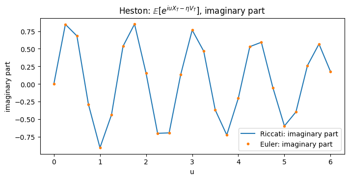
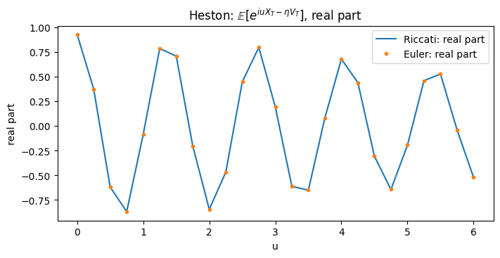
Note that some discrepancy is expected because of Monte Carlo sampling error, Euler time-stepping bias and numerical ODE error.
Increasing the number of paths primarily reduces sampling noise, while decreasing the time steps improves discretization error.
7.2. Transform methods and option pricing
Carr–Madan Option PricingWe now spend some time understanding how to price European call options using the characteristic function of the terminal log-price, , as this is useful when that function can be found but the probability distribution of is difficult to work out.
Firstly, we consider , the asset price at maturity and , the strike. A call option pays , so its discounted price is:
Since we have , can take any value, so we have . We therefore work with (and not ) since the Fourier transform integrates over .
As , tends to zero, so the call pays almost the entire asset price (), so does not decay at the left of the real line (but note that its Fourier integral is not absolutely integrable there).
We now introduce the damped call price as:
Intuition: as , goes to zero, so we remove the nondecaying left tail, and the condition ensures that damping does NOT cause integrability problems.
With the damped call price, we can write the Fourier transform, substitute the definition of , and then the call price formula as:
We now define , so we have . We now interchange the integral and the expectation and write:
Given this, we fix the terminal log-price and calculate
As above, this is nonzero only if , so we can substitute and distribute :
where the extra in comes from the fact that .
Since , tends to zero if , so we have , which implies:
If we multiply by , we have
We now integrate the second term similarly, so we have:
We now combine the results:
and we immediately notice that we can simplify the expression in parentheses:
So we have:
We now replace by the random value , substitute the integral into the damped call price and, since the denominator does NOT depend on , we can extract it from the expectation:
We now recall that the characteristic function is , so we want to express the numerator using . We therefore choose
Finally, we obtain the transformed call price
If we multiply the factors:
Finally, we recover the call price by Fourier inversion.
Our transform uses the positive sign , so its inverse uses the negative sign . Since is real-valued, we have conjugate symmetry:
Adding them together gives us the real part:
and, if we undo the damping since , we finally have:
This is the Carr–Madan inversion formula.
Discrete (DFT) and Fast Fourier Transform (FFT) in the Carr–Madan formula
To use the Carr–Madan formula mentioned before, we need to approximate an integral. To do this, we need to replace the integral with a sum, so if we choose equally spaced frequencies for , we can write:
where are numerical integration weights.
Given complex numbers , we define the discrete Fourier transform (DFT) as the array
where identifies the input and the output value . The idea is that for each we multiply every by a complex oscillating factor and sum the results.
However, each requires the sum of terms, so, since we have outputs, we have complexity .
The fast Fourier transform (FFT), on the other hand, does the same more efficiently.
We indeed assume that is a power of 2, so we start from:
and we define , so we can write:
The even indices are , while the odd indices are , so we have:
where the second equality comes from .
Since we have that , the two sums are DFTs of size defined by:
and if we consider that is the transform of the even indices and of the odd, we can express one large transform in terms of two smaller ones:
Furthermore, for , the smaller DFTs repeat after indices and, since , we have:
So, for the same and , we have two outputs:
so the FFT applies this split to smaller transforms until we reach arrays of size 1. Doing so, there are splitting levels and, at each level, the total work is proportional to , therefore the total cost is .
We now come back to the DFT in Carr–Madan and the discretized integral
The idea is to choose frequency and strike grids so that becomes from the DFT.
Indeed, we choose the grid and we choose equally spaced log-strikes:
Note that are equally spaced but the corresponding actual strikes are not.
If we substitute and we get:
We then choose the grid spacings such that , so we have exactly the DFT factor:
Define now the inputs as:
so the sum in the pricing formula becomes exactly a DFT sum
Taking the real part and undoing the damping gives the call prices at the log-strike grid points:
8. Strong approximation of Stochastic Differential Equations
8.1. Coefficient regularity and convergence
In this chapter, we spend some time understanding how to numerically approximate stochastic differential equations of the form:
where is the unknown state, the drift, the diffusion coefficient and a Brownian motion.
Growth properties
Growth conditions describe how quickly a function can become large as inputs move and this matters because coefficients that grow too fast can make solutions or their moments difficult to handle.
Linear GrowthA function has at most linear growth if, for some we have:
The constant allows to be nonzero, otherwise the property would not be satisfied.
Intuition: doubling the input can increase the upper bound of the function by a factor of two.
Quadratic growthA function has at most quadratic growth if
Of course, every linear growth function is also of quadratic growth.
Polynomial growthA function has at most polynomial growth if, for some we have:
Intuition: if has polynomial growth and has sufficiently many finite moments, then is finite (this will be important when testing for weak convergence).
Growth properties of derivatives Global Lipschitz continuityA function is globally Lipschitz if there is an such that, for all :
For a differentiable scalar function, a bounded derivative gives this property. By the mean value theorem we indeed have:
Note that Lipschitz continuity implies linear growth (but the converse is false). If we indeed set we have:
Polynomially growing derivativesA function is times continuously differentiable with at most polynomially growing derivatives when and its -th derivative satisfies the polynomial growth condition (note that in this case the lower derivatives also have polynomial growth) Infinitely differentiable with polynomially growing derivatives
is infinitely differentiable with at most polynomially growing derivatives if and every derivative has at most polynomial growth (note however that the bound can be different for each derivative).
Strong convergence
Let be the target process and its approximation using steps. At time , we can write the error as
We can say that there is strong convergence if, for we have .
Intuition: for , the absolute average error tends to zero, for the root mean square error tends to zero and larger penalizes large errors more heavily.
Furthermore, we say that convergence has a strong order if there is such that:
Almost sure convergence
We say that converges to almost surely if
We say that converges to almost surely of order if there is a finite random variable such that, almost surely, for all
Note that there's an important difference between strong order convergences:
- strong convergence uses a deterministic constant
- almost sure order uses a path-dependent constant.
Convergence in probability
converges to in probability if for every we have, for :
Intuition: up to approximation, the chance of making an error larger than becomes small.
Note also that both almost sure convergence and strong convergence imply convergence in probability (but the reverse does not hold).
Numerically weak convergence
Weak convergence focuses on statistics of the solution. For each smooth test function , we say that converges numerically weakly at time to if:
Intuition: while strong convergence tests if the paths are close, weak convergence tests if the statistics of the path (for example expected value) are similar.
Similarly we have weak convergence of order if for every admissible there is a such that:
8.2. Euler–Maruyama approximation
Euler-Maruyama schemeWe now consider an interval of length . The exact solution of the SDE is
If we approximate both coefficients by their values at the start of the interval we have:
so we can write
so we can write:
Euler-Maruyama approximationIf we now consider , and the previous scheme can be written as:
Intuition: we take the previous state and we apply a deterministic drift increment and a random increment .
Furthermore, for we can write:
so the Linear interpolated Euler approximation (i.e. the continuous piecewise linear version of the Euler-Maruyama approximation) is
Theorem: Strong Convergence of Euler-Maruyama
We assume , in and global Lipschitz bounds, i.e.
Let also be the solution and the linearly interpolated Euler approximation with steps. We define
Then we have that:
Intuition: at every , we take errors across the sample paths, we take the worst error and we say that the worst fixed time error decreases at least as order .
Theorem: Uniform strong convergence
Under the stated global-Lipschitz and moment assumptions, the linearly interpolated scheme satisfies
where the constant does not depend on .
Note that the previous theorem focuses on .
In the first expression, choose one time and average across paths; then find the worst time. In the second, find the worst time separately for each path, then average. Different paths may have their largest errors at different times.
Indeed, we have that: