Machine Learning in Finance and Insurance

The following notes come from the course Machine Learning in Finance and Insurance, taught at ETH Zurich by Patrick Cheridito, Professor of Mathematics at ETH Zurich and Director of RiskLab Switzerland.

Feel free to reach out to me with any comments, clarifications, or corrections.

Index

• Basic Notions of Statistical Learning
• Linear Regression
• Gradient Descent
• Logistic Regression
• Kernel Methods
• Neural Networks
• Classification and Regression Trees
• Bagging and Random Forests
• Gradient Boosted Trees
• Dimensionality Reduction and Autoencoders
• Generative Models

The following notes come from the course Machine Learning in Finance and Insurance, taught at ETH Zurich by Patrick Cheridito, Professor of Mathematics at ETH Zurich and Director of RiskLab Switzerland.

Feel free to reach out to me with any comments, clarifications, or corrections.

1 Basic Notions of Statistical Learning

Firstly, we remember that a $\sigma$-algebra $\mathcal{F}$ is a non-empty collection of subsets of $\Omega$ that contains $\Omega$ itself and is closed under complementation and countable unions, i.e. it satisfies the following:

• contains the whole space $\Omega \in \mathcal{F}$
• closed under complementation: $\text{If }A\in \mathcal{F},\text{ then }{A}^c=\Omega \setminus A\in \mathcal{F}$
• it is closed under countable unions: $\text{If }{A}_1,A_2,A_3,\cdots \in \mathcal{F},\text{ then }{\bigcup }_{n=1}^{\infty }{A}_n\in \mathcal{F}$

From this definition, we provide some examples:

• Trivial $\sigma$-algebra: $\mathcal{F}=\{\varnothing ,\Omega \}$ (the smallest $\sigma$-algebra)
• Power set: $\mathcal{F}=\mathcal{P}(\Omega )$ (collection of all subsets of $\Omega$, the largest possible $\sigma$-algebra)
• Borel $\sigma$-algebra (smallest $\sigma$-algebra generated by all open sets in $\mathbb{R}$, it is the essential foundation for measure theory and real analysis)

Intuition: in $\mathbb{R}$, consider all the intervals $(a,b)$ and perform all three actions that define the $\sigma$-algebra (complements, countable unions, countable intersections, where the last one nicely derives from the definition of $\sigma$-algebra): the resulting set is the Borel $\sigma$-algebra $\mathcal{B}(\mathbb{R})$ and represents every subset of $\mathbb{R}$ that can be obtained using standard mathematical operations.)

We also recall that a function $f:X\to Y$ is Borel measurable if:

Intuition: if the preimage of every Borel set in $Y$ is a Borel set in $X$.

Consider the following:

• a probability space $(\Omega ,\mathcal{F},\mathbb{P})$, i.e.:
  • a non-empty set $\Omega$, the sample space
  • $\mathcal{F}$, a $\sigma$-algebra of subsets of $\Omega$,
  • a probability measure $\mathbb{P}:\mathcal{F}\to [0,1]$
• a feature space $\mathcal{X}\subseteq {\mathbb{R}}^d$ with Borel $\sigma$-algebra ${\mathbb{B}}_{\mathcal{X}}$ (example: $\mathcal{X}={\mathbb{R}}^m\times \{1,2,\dots ,n\}\times \mathbb{N}$)
• a closed or open target space $\mathcal{Y}\subseteq {\mathbb{R}}^k$ with Borel $\sigma$-algebra ${\mathbb{B}}_{\mathcal{Y}}$ (example: $\mathcal{Y}=\mathbb{R}$)
• some random elements $X:\Omega \to \mathcal{X}$ (inputs), $Y:\Omega \to \mathcal{Y}$ (outputs)

We then consider ${\rho }_X,{\rho }_Y,\rho$ the distributions of $X,Y,(X,Y)$ and ${\rho }_{Y\mid X}$, that is the regular conditional distribution of $Y$ given $X$, that is:

• $\forall x\in \mathcal{X}:{\rho }_{Y\mid X}(\cdot \mid x)$ is a probability measure on $\mathcal{Y}$
• $\forall B\in {\mathbb{B}}_{\mathcal{Y}}$, $x\mapsto {\rho }_{Y\mid X}(B\mid x)$ is ${\mathbb{B}}_{\mathcal{X}}$-measurable
• $\forall B\in {\mathbb{B}}_{\mathcal{Y}}$, $\mathbb{E}[1_B(Y)\mid X]={\rho }_{Y\mid X}(B\mid X)$ $\mathbb{P}$-almost surely.

Then, it follows, for all $\rho$-integrable $h:\mathcal{X}\times \mathcal{Y}\to \mathbb{R}$, we have the disintegration of $\rho$:

We now go back to the prediction problem: we want to find a measurable function $f:\mathcal{X}\to \mathcal{Y}$ s.t. $f(X)\approx Y$, i.e. a function that allows us to minimize the expected loss (also called risk), defined as:

for a measurable loss function $\ell :\mathcal{Y}\times \mathcal{Y}\to {\mathbb{R}}_{+}$.

Then, in machine learning, it is common to solve the empirical loss minimization problem!

Let $\bar{f}:\mathcal{X}\to \mathcal{Y}$ be a measurable function such that, for ${\rho }_X$-almost every $x\in \mathcal{X}$, $\bar{f}(x)$ minimizes

Then

for every measurable function $f:\mathcal{X}\to \mathcal{Y}$.

Note that $\bar{f}(x)$ is the ideal predictor we would use if we knew the true conditional distribution of $Y$ given $X=x$. For each $x\in \mathcal{X}$, if we predict a value $w\in \mathcal{Y}$, the conditional expected loss is

The function $\bar{f}$ chooses the prediction that minimizes this conditional risk:

From now on, we suppose these assumptions from the lemma hold and we call:

• $\bar{f}$ regression function (or, more generally, the Bayesian-optimal predictor)
• $\mathbb{E}[\ell (\bar{f}(X),Y)]$ irreducible error (even with the exact conditional distribution, randomness in $Y$ given $X$ can prevent perfect prediction)

We consider now the following example with $\mathcal{Y}\subseteq \mathbb{R}$, $\ell (w,y)=(w-y{)}^2$ and a random variable $Z$ with $\mathbb{E}[Z^2]<\infty$.

Then, $\forall w\in \mathbb{R}$:

so the mapping $w\mapsto \mathbb{E}[(w-Z{)}^2]$ is strictly convex with:

• a unique minimizer $w=\mathbb{E}[Z]$ (under square loss: the best constant prediction of $Z$ is its mean)
• a minimal value of $\mathrm{Var}(Z)=\mathbb{E}[(Z-\mathbb{E}[Z]{)}^2]=\mathbb{E}[Z^2]-(\mathbb{E}[Z]{)}^2$ (the minimal possible error is its variance)

We now assume $\mathbb{E}[Y^2]<\infty$, by disintegration we obtain:

Therefore we have

for ${\rho }_X$-almost every $x\in \mathcal{X}$. By the Cauchy–Schwarz inequality, this also implies

for ${\rho }_X$-almost every $x\in \mathcal{X}$.

The conditional risk under squared loss is then:

The second term does not depend on $w$, and the first one is minimized when:

Therefore, the unique minimizer is:

Then, we easily obtain the least-squares regression function and its minimum loss (risk):

and

We now consider $\mathcal{Y}\subseteq \mathbb{R}$ and a loss function $l(w,y)=l_{\alpha }(y-w)$, with $\alpha \in (0,1)$ and the pinball loss function defined as:

In this formula, $\alpha$ is the quantile we want to predict and it determines the asymmetry of the loss. Indeed, in the pinball loss function, the penalty is proportional to $1-\alpha$, therefore:

• for $\alpha >1/2$: underprediction is penalized more
• for $\alpha <1/2$: overprediction is penalized more
• for $\alpha =1/2$: both directional errors have the same cost

We firstly note that:

• ${\partial }_{+}{\ell }_{\alpha }(\mu )=\alpha -1_{\{\mu <0\}}$
• ${\partial }_{-}{\ell }_{\alpha }(\mu )=\alpha -1_{\{\mu \le 0\}}$

We now consider a random variable $Z$ with $\mathbb{E}[|Z|]<\infty$. In this case, $\mathbb{E}[{\ell }_{\alpha }(Z-w)]$ is convex in $w$ and:

• ${\delta }_{+}\mathbb{E}[{\ell }_{\alpha }(Z-w)]=\mathbb{P}[Z\le w]-\alpha$
• ${\delta }_{-}\mathbb{E}[{\ell }_{\alpha }(Z-w)]=\mathbb{P}[Z<w]-\alpha$

So $w$ is a minimizer of $\mathbb{E}[{\ell }_{\alpha }(Z-w)]$ if and only if $\mathbb{P}[Z<w]\le \alpha$ and $\mathbb{P}[Z\le w]\ge \alpha$, if and only if $w$ is an $\alpha$-quantile of $Z$.

Now let $q_{\alpha }(x)$, for $x\in \mathcal{X}$, be an $\alpha$-quantile of the conditional distribution ${\rho }_{Y\mid X}(\cdot \mid x)$. Then we have:

• $\bar{f}(x)=q_{\alpha }(x)$
• $\mathbb{E}[\ell (\bar{f}(X),Y)]=\mathbb{E}[{\ell }_{\alpha }(Y-q_{\alpha }(X))]$ (quantile regression)

For the special case $\alpha =1/2$, $q_{1/2}(Z)$ is a median of $Z$, and $\mathbb{E}[{\ell }_{1/2}(Y-q_{1/2}(X))]=\frac{1}{2}\mathbb{E}[|Y-q_{1/2}(X)|]$ is the minimal MAE.

Let $(X_i,Y_i)$ with $i=1,\dots ,m$ be independent copies of $(X,Y)$, called training data.

The empirical loss/risk of a measurable function $f:\mathcal{X}\to \mathcal{Y}$ is $\frac{1}{m}{\sum }_{i=1}^m\ell (f(X_i),Y_i)\approx \mathbb{E}[\ell (f(X),Y)]$. In the case of $\mathbb{E}[{\ell }^2(f(X),Y)]<\infty$, we can write:

and we can call this weak law of large numbers.

Intuition: with the training data growing, variance approaches zero.

A hypothesis class is a family $\mathcal{H}$ of measurable functions $f:\mathcal{X}\to \mathcal{Y}$, e.g.:

• all affine functions (i.e. weighted sums of features $X_i$)
• 2nd order polynomials
• splines (local polynomial pieces joined together, producing a smooth flexible curve)
• trees (sequential if-then rules with piecewise constant regions)
• support vector machines (separate classes with a maximum-margin boundary)
• neural networks (several nonlinear transformations)

Ideally, we would like to minimize $\mathbb{E}[\ell (f(X),Y)]$ over all measurable functions $f$.

However, in practice, we try to find a numerical solution ${\hat{f}}_m$ to the empirical loss minimization problem:

Note that ${\hat{f}}_m$ can be produced by either:

• a deterministic algorithm, in the form ${\hat{f}}_m=\hat{\varphi }(\cdot ,(X_i,Y_i{)}_{i=1}^m)$, where $\hat{\varphi }$ is a measurable function of the training data;
• a stochastic optimization algorithm, in the form ${\hat{f}}_m=\hat{\varphi }(\cdot ,(X_i,Y_i{)}_{i=1}^m,V)$, where $V$ is a random element independent of the training data and $\hat{\varphi }$ is measurable (note that a stochastic algorithm can produce different results with the same training data due to the presence of the noisy term $V$)

Given the numerical solution ${\hat{f}}_m$, we now formalize the expected loss decomposition for the square loss function.
We first define the conditional expected loss given that $X=x$:

If we define:

• ${\hat{f}}_m^{\mathrm{avg}}(x)=\mathbb{E}[{\hat{f}}_m(x)]$
• $\bar{f}(x)={\int }_{\mathcal{Y}}y{\rho }_{Y\mid X}(dy\mid x)=\mathbb{E}[Y\mid X=x]$

then we can write the conditional expected loss as:

The first term is the conditional bias squared, the second term is the conditional variance, and the last term is the conditional irreducible error.

Furthermore, the expected loss is (the calculations are omitted for economy of space; readers are encouraged to compute them by hand):

The first term is the average bias squared, the second term is the average variance, and the last term is the irreducible error.

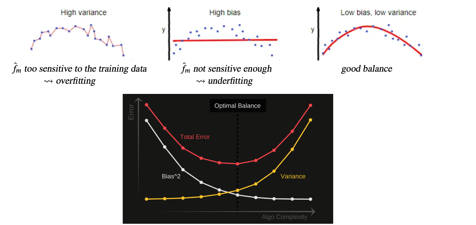
For a given size $m$ of the training set, we can then define:

• the bias as the distance of the average prediction function ${\hat{f}}_m^{\mathrm{avg}}$ from the true regression function $\bar{f}$
• the variance as the variation of the data-dependent (noisy) prediction function ${\hat{f}}_m$

and... of course, we should aim for a good balance between them!

If we consider the same square loss function, a training data set $(X_i,Y_i)$, with $i=1,\dots ,m$, and a test dataset $(X_i,Y_i)$, with $i=m+1,\dots ,m+n$, and ${\hat{f}}_m$ a prediction function trained on the training data, we can define the in-sample goodness of fit $R^2$ as:

where

• SSR = ${\sum }_{i=1}^m(Y_i-{\hat{f}}_m(X_i){)}^2$ (sum of squared residuals)
• SST = ${\sum }_{i=1}^m(Y_i-{\bar{Y}}_{\mathrm{train}}{)}^2$, with ${\bar{Y}}_{\mathrm{train}}=\frac{1}{m}{\sum }_{i=1}^m{Y}_i$ (total sum of squares)

Note that, with the same approach, we can define the out-of-sample $R^2$, using $Y_i$ and ${\hat{f}}_m(X_i)$ from the testing dataset.

As an obvious intuition, $R^2$ measures prediction power (higher is therefore better!).

If $\mathcal{H}$ is not flexible enough to approximate $f$ well (i.e. the hypothesis class does not contain the ideal predictor $\bar{f}$), we can incur an approximation error, that measures the limitation of the current model family itself in comparison with the ideal model and it is defined as:

If the empirical loss minimization problem, i.e. $\min \frac{1}{m}{\sum }_{i=1}^m\ell (F(X_i),Y_i)$, has a solution, we call that solution ${\hat{f}}_m^{\mathcal{H}}\in \mathcal{H}$ (note that in this case ${\hat{f}}_m^{\mathcal{H}}$ is random, since it depends on $(X_1,Y_1),\dots ,(X_m,Y_m)$).

If ${\hat{f}}_m^{\mathcal{H}}$ exists, it is random because it depends on the random training sample. In this case, its sampling error (estimation error) is the difference between its true loss and the population loss available in $\mathcal{H}$ (it results from minimizing the empirical loss instead of the expected loss; it typically decreases with increasing sample size $m$), i.e.:

Consider a numerical solution ${\hat{f}}_m$ of ${\inf }_{f\in \mathcal{H}}\frac{1}{m}{\sum }_{i=1}^m\ell (f(X_i),Y_i)$, with:

• ${\hat{f}}_m=\varphi (\cdot ,(X_i,Y_i{)}_{i=1}^m,V)$
• measurable $\varphi$ and a $\mathcal{V}$-valued random element $V$ independent of $(X,Y)$.

We can then define the direct optimization error as:

Note that the first term is the empirical loss achieved by the numerical solution, the second is the lowest empirical loss achievable by any function in $\mathcal{H}$. Note also that this error is different from the sampling error:

• the optimization error measures failure to solve the training problem
• the sampling error measures the gap between training performance and test data performance

Once we have defined the previous metrics, we can define the following:

For a given $m$ and an increasing $\mathcal{H}$ (i.e. the set of models we can choose from is increasing):

• approximation error is decreasing
• sampling error tends to increase
• there's a tradeoff between approximation error and sampling error (similar to the bias-variance tradeoff)
• for small data $\mathcal{H}$ should be simple (and for big data, it can be complex!)

Once we have defined ${\hat{f}}_m$, we condition on it and so it is no longer random.

If we consider training and test data sets, we can define:

If $E_{\mathrm{tr}}$ is significantly smaller than $E_{\mathrm{te}}$, the model is most likely overfitted.

We can then calculate the sample variance:

which, if $\mathbb{E}[{\ell }^2({\hat{f}}_m(X),Y)\mid {\hat{f}}_m]<\infty$, follows the Law of Large Numbers and converges, as $n\to \infty$, to $\mathrm{Var}(\ell ({\hat{f}}_m(X),Y)\mid {\hat{f}}_m)$.

Furthermore, by the Central Limit Theorem, we have:

Therefore, we have the following property:

That is a confidence interval with confidence level $1-\alpha$, where $q_{1-\alpha /2}$ is the $(1-\alpha /2)$-quantile of the standard normal distribution.

We now come back to the overfitting problem: what can we do about it? Firstly, we can reduce the complexity of the hypothesis class, i.e. by considering simpler models. Alternatively, we can regularize the empirical loss minimization problem by penalizing the complexity of potential prediction functions $f\in \mathcal{H}$, which, practically speaking, means:

for hyperparameters ${\lambda }_1\ge 0$ (strength of the Lasso penalty), ${\lambda }_2\ge 0$ (strength of the ridge penalty).

We call ${\lambda }_1\Vert f{\Vert }_1$ LASSO and ${\lambda }_2\Vert f{\Vert }_2^2$ ridge regression; together, they compose the elastic net.

In general, LASSO penalizes the absolute value of the coefficients and can set them to zero, and it is defined as:

Therefore, LASSO performs feature selection, i.e. limits the features with lower explanatory power.

On the other hand, ridge regression defines a penalty equal to:

It discourages large coefficients but does not make them exactly zero; it smoothly shrinks them around zero.

Ridge regression can be useful when features are correlated. In this situation, LASSO may select one feature and discard another similar one, while ridge tends to distribute the coefficients across them.

When both penalties are present the method is called elastic net, since it combines LASSO's ability to set coefficients to zero and ridge regression's shrinkage of correlated features.

2 Linear Regression

3 Gradient Descent

4 Logistic Regression

5 Kernel Methods

6 Neural Networks

7 Classification and Regression Trees

8 Bagging and Random Forests

9 Gradient Boosted Trees

10 Dimensionality Reduction and Autoencoders

11 Generative Models