Principles of Econometrics

Index

Introduction to Statistics and Econometrics
Simple Regression Analysis
Multiple Regression Analysis: Basics
Multiple Regression Analysis: Inference
Multiple Regression Analysis: Further Issues
Heteroskedasticity and Other Problems
Time Series Data
Panel Data
Instrumental Variables

1 Introduction to Statistics and Econometrics

Econometrics is the use of statistical methods to analyze economic data, starting typically from non-experimental data.

Common goals of econometric analysis are:

estimating relationships between variables
testing economic theories and hypotheses
evaluating and implementing government and business policy

Structure of Econometric Data

Cross sectional data
- observations that represent individuals, firms, cantons, countries (normally, but not necessarily, at one point in time).
- observations are drawn randomly from a population (if not, we have a sample-selection problem)
Time Series Data
- observations represent periods in time
- observations are consecutive and hence not random
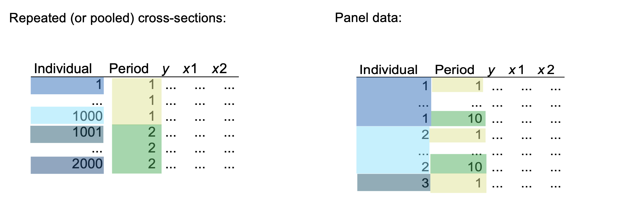
Pool Cross-Sections
- at least two cross sections are combined in one data set
- cross sections are drawn independently of each other
- can often be treated similar to a normal cross section
Panel (or longitudinal data)
- cross-sectional units followed over time
- panel data have a cross-sectional and time series dimension
- useful to account for time-invariant unobservables and for modeling lagged responses

Causality

The definition of causal effect of $x$ on $Y$ is: "how does variable $y$ change if variable $x$ is changed, but all other factors are held constant?
(This concept is called Ceteris Paribus).

Simply establishing a relationship (correlation) between variables can be misleading (important distinction between correlation and causation!)

There are multiple types of experiments that allow answering causal questions:

Randomized controlled trials (RCT)
Natural experiments

Probability Review: Distributions

Chi-Square Distribution

Let $Z_{i}$ be $n$ independent random variables with $Z_{i} \sim N (0, 1)$ , then

X = i = 1 \sum n Z_{i}^{2}

has a chi-square distribution with $n$ degrees of freedom and we write $X \sim χ_{n}^{2}$ .

t-Distribution

Let $Z \sim N (0, 1)$ and $X \sim χ_{n}^{2}$ , then

T = Z / X / n

has a t-distribution with $n$ degrees of freedom and we write $T \sim t_{n}$ .

F-Distribution

Let $X \sim χ_{k}^{2}$ and $Y \sim χ_{l}^{2}$ and assume $X, Y$ independent, then:

F = \frac{( X / k )}{( Y / l )}

has an F-distribution with $(k, l)$ degrees of freedom and we write $F \sim F_{k, l}$ .

Central Limit Theorem

The standardized average $Z$ of any population with mean $μ$ and variance $σ^{2}$ is asymptotically $N (0, 1)$ distributed, or, in other words:

Z = (\overset{y}{ˉ} - μ) / (σ / n) \sim N (0, 1)

Law of Large Numbers

Let $y_{1}, \dots, y_{n}$ be independent, identically distributed random variables with mean $μ$ , then:

n \to \infty lim (\frac{1}{n} i \sum n y_{i}) = μ

2 Simple Regression Analysis

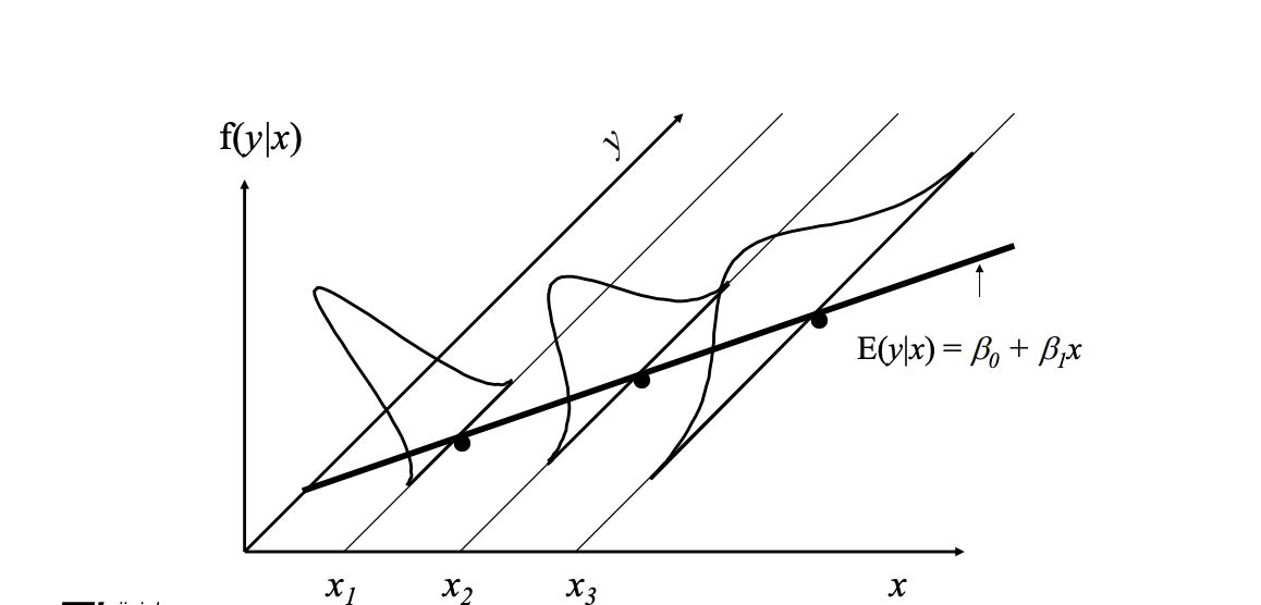
How can we use the data to describe economic relations or behaviors?

y = β_{0} + β_{1} x + μ

$y$ : dependent variable (outcome variable)
$x$ : independent variable (regressor, covariate, control variable, "the cause")
$μ$ : error term (disturbance)
- it represents strictly unpredictable random behaviors, unspecified or unobserved factors or an approximation error if the relation is not perfectly linear.
$β_{0}$ : intercept parameter
$β_{1}$ : slope parameter

We start now with Population Modelling and consider the following assumptions:

SLR.1: Linear parameters
- in the population model the following relation holds: $y = β_{0} + β_{1} x + μ$
SLR.2: Random sampling
- we have a random sample of size $n$ of random variables $(x, y)$
SLR.3: Sample variation in the explanatory variable
- the sample outcomes on $x$ are not all the same value
SLR.4: Zero Conditional Mean

E [μ ∣ x] = E [μ] = 0

or, in other words, for every slice of the population determined by $x$ , the average of $μ$ is equal to the population average $μ$ (which is zero).
This also implies:

E [y ∣ x] = β_{0} + β_{1} x

also called the Population Regression Function.

Population Model

We now derive the Ordinary Least Squares (OLS).

Intuition: we estimate the population parameters from a data sample of two random variables.

Let ${(x_{i}, y_{i})} : i = 1, \dots, n$ denote a random sample of size $n$
scatter plot in a $(x, y)$ system
the regression equation $y_{i} = β_{0} + β_{1} x_{i} + μ_{i}$ allocates to each $x_{i}$ a value $y_{i}$ including a disturbance term $μ_{i}$ .

But how can we derive the estimates for $β_{0}, β_{1}$

We firstly rely on the SLR.4 assumption to derive two equations:

E [μ] E [u ∣ x] = 0 ⟹ E [y - β_{0} - β_{1} x] = 0 = 0 ⟹ Cov [x, u] = E [xμ] - E [x] E [μ] = = E [xμ] = E [x (y - β_{0} - β_{1} x)] = 0

These are called populatio moment restrictions

Using then the sample moments from the population, we can get estimates of the population moments.

Recall:

$\sum_{i} (y_{i} - β_{0} - β_{1} x_{i}) / n = 0 (1)$
$\sum_{i} x_{i} ((y_{i} - β_{0}) - β_{1} x_{i}) / n = 0 (2)$

we rewrite $(1)$ as: $b_{0} = \overset{y}{ˉ} - b_{1} \overset{x}{ˉ}$ , then we plug into $(2)$ and solve for $b_{1}$ :

b_{1} = \frac{\sum _{i = 1}^{n} ( x _{i} - x ˉ ) ( y _{i} - y ˉ )}{\sum _{i = 1}^{n} ( x _{i} - x ˉ ) ^{2}}

Finally, we can easily put back $b_{1}$ into the first equation and derive $b_{0}$ .

Intuition: the slope estimate is the sample covariance between $x$ and $y$ , divided by the sample variance of $x$ .

if $x, y$ are positively correlated, the slope will be positive.
if $x, y$ are negatively correlated, the slope will be negative.

Moreover, intuitively, the OLS is fitting a line through the sample points such that the sum of squared residuals is as small as possible.

Algebraic Properties of OLS:

the sum of the OLS residuals is zero.
the sample average of the OLS residuals is zero.
the sample covariance between the regressors and the OLS residuals is zero.
the OLS regression line always goes through the mean of the sample.

Moreover, we notice that each observation $y_{i}$ is made up of an explained $\overset{y}{^}_{i}$ and unexplained part $\overset{u}{^}_{i}$ ( $y_{i} = \overset{y}{^}_{i} + \overset{u}{^}_{i}$ ).

Using this terminology, we can define:

$Sum of Squares Total (SST) = \sum_{i} (y_{i} - \overset{y}{ˉ})^{2}$
$Sum of Squares Explained (SSE) = \sum_{i} (\overset{y}{^}_{i} - \overset{y}{ˉ})^{2}$
$Sum of Squares Residuals (SSR) = \sum_{i} (\overset{u}{^}_{i})^{2}$

To understand how well does the sample fit the regression line, we define:

R^{2} = \frac{SSE}{SST} = 1 - \frac{SSR}{SST}

Be aware that, the term linear in a OLS model does not mean a linear relationship between the variables, but a model in which the parameters enter the model in a linear way.
The following are all linear models (in the parameters):

$y = β_{0} + β_{1} ln (x) + μ$
$ln (y) = β_{0} + β_{1} x + μ$
$y = β_{0} + β_{1} (\frac{1}{x}) + μ$

Implication of the Simple Linear Regression

OLS is unbiased (the proof depend on the 4 assumptions, if any fails, the OLS is not necessarily unbiased)
The sampling distibution of our estimates is centered around the true parameter

But, following the second implication, how likely is it that the true slope is slightly larger, smaller or zero?

This question can be translated into another assumption:

SLR.5 Homoskedasticity: assume $Var [μ ∣ x] = σ^{2}$

Using then the Homoskedasticity assumption, we can derive the variance of $b_{1}$ .

Var [μ ∣ x] = E [μ^{2} ∣ x] - E [μ ∣ x]^{2} = E [μ^{2} ∣ x] = E [μ^{2}] = Var [μ] = σ^{2}

Hence, $σ^{2}$ is also the unconditional variance, called the error variance.

We can then use this formula to find the variance of $b_{1}$ :

Var (b_{1}) = \frac{σ ^{2}}{\sum _{i = 1}^{n} ( x _{i} - x ˉ ) ^{2}} = \frac{σ ^{2}}{SS T _{x}}

the larger the error variance $σ^{2}$ , the larger the variance of the slope estimate.
the large the variability in the $x$ ( $SS T_{x}$ ), the smaller the variance of the slope estimate.

Finally, starting from the residuals $\overset{u}{^}_{i}$ , we can form an unbiased estimate of the error variance (often called the mean square error (MSE)), denoted by $s^{2}$ :

s^{2} = (n - 2)^{- 1} i \sum \overset{u}{^}_{i}^{2} = \frac{SSR}{n - 2}

Intuition: $σ^{2}$ is the truth; $s^{2}$ is our best guess based on the sample we have.

Moreover, we divide by $(n - 2)$ because, estimating $b_{0}, b_{1}$ , we lost 2 degrees of freedom.

3 Multiple Regression Analysis: Basics

The key problem with simple linear regression is that the assumption $E [u ∣ x] = E [u] = 0$ is often problematic.

Consider, for example, that the true population model is:

wage wage = β_{0} + β_{1} education + β_{2} IQ + μ = β_{0} + β_{1} education + v

The previous assumption states that the error term $v = β_{2} IQ + μ$ has $0$ (zero) expected value (no trend) or, in other words, $IQ$ does not correlate with the $wage$ .

This causes $β_{1}$ to be biased compared to the "true parameter", so it doesn't measure the causal effect of education to wage.

Thus, instead of assuming that multiple variables are uncorrelated with the output variable, the multiple regression model allows to include them directly in the model.

y = β_{0} + β_{1} x_{1} + β_{2} x_{2} \dots β_{k} x_{k} + μ

$β_{0}$ is still the intercept
$β_{0} \dots β_{k}$ are the slope parameters
$μ$ is the error term.

We still need a zero conditional mean: $E [u ∣ x_{1} \dots x_{k}] = 0$ , that means, in other words, that all the factors that influence the outcome are included in the model.

In order to estimate the parameters, we still use the Ordinary Least Squares method and we minimize the residuals:

β_{0} \dots β_{k} min i \sum (y_{i} - β_{0} - β_{1} x_{1} \dots β_{k} x_{k} - μ)^{2}

leading to $k + 1$ conditions to derive $k + 1$ parameters.

The estimate model $\overset{y}{^} = b_{0} + b_{1} x_{1} + b_{2} x_{2} \dots b_{k} x_{k} + μ$ alloqs a ceteris paribus interpretation, that means that a change in $x_{1}$ , $Δ x_{1}$ , leads to a change in $y$ given by $b_{1} Δ x_{1}$ , keeping all the other $x_{i}$ fixed.

Frisch-Waugh-Lovell (FWL) Theorem

Given a multiple (dual for example) regression model $y = β_{0} + β_{1} x_{1} + β_{2} x_{2} + μ$ , the coefficient $β_{1}$ can be found in 2 steps:

Regress $x_{1}$ on $x_{2}$ :

x_{1} = α_{0} + α_{1} x_{2} + u

Save then the residuals $\overset{r}{^}_{1} = x_{1} - \overset{x}{^}_{1}$ . This represents the part of $x_{1}$ not correlated with $x_{2}$ .

Regress $y$ on the residuals:

y = γ \overset{r}{^}_{1} + e

The resulting coefficient $γ$ will be identical $b_{1}$ of the original model.

The previous definition of $R^{2}$ is still valid, but we can add the following remarks:

$R^{2}$ is the squared correlation coefficient between $y$ and the predicted $\overset{y}{^}$ .
$R^{2}$ never decreases when adding independent variables to a regression (usually will increase).
Because it increases changing the number of parameters, it NOT a good measure to compare different models.

As in the simple regression model, we can formalize the assumptions for the multiple one:

MLR.1: Linear in parameters
in the population model the following relation holds:
$y = β_{0} + β_{1} x_{1} + \dots + β_{k} x_{k} + μ$
MLR.2: Random sampling
we have a random sample of size $n$ :
${(y_{i}, x_{i 1}, \dots, x_{ik})}_{i = 1}^{n}$
MLR.3: No perfect collinearity (sample variation in explanatory variables) no explanatory variable is an exact linear combination of the others, and each regressor has variation in the sample.
MLR.4: Zero Conditional Mean $E [μ ∣ x_{1}, \dots, x_{k}] = 0$
or, for every slice of population determined by $(x_{1}, \dots, x_{k})$ , the average of $μ$ is zero.

This also implies:
$E [y ∣ x_{1}, \dots, x_{k}] = β_{0} + β_{1} x_{1} + \dots + β_{k} x_{k}$
also called the Population Regression Function.

Then, we can derive the following:

Implication 1: Unbiasedness of OLS

Under the previous assumptions, the OLS estimator is unbiased: $E [b_{i}] = β_{i}$ .

If we include irrelevant variables in our model, the OLS estimator remains still unbiased.
If we exclude relevant variables, OLS will usually be biased.

Let's suppose the true model is:

y = β_{0} + β_{1} x_{1} + β_{2} x_{2} + μ

but our model is:

y = γ_{0} + γ_{1} x_{1} + v

and we actually estimate:

y = c_{0} + c_{1} x_{1} .

The slope parameter will then be:

c_{1} = \frac{\sum _{i = 1}^{n} ( x _{i} - x ˉ ) ( y _{i} - y ˉ )}{\sum _{i = 1}^{n} ( x _{i} - x ˉ ) ^{2}}

Recall that the numerator is:

= = i = 1 \sum n (x_{i 1} - \overset{x}{ˉ}_{1}) (y_{i} - \overset{y}{ˉ}) = i = 1 \sum n (x_{i 1} - \overset{x}{ˉ}_{1}) (β_{0} + β_{1} x_{i 1} + β_{2} x_{i 2} + u_{i} - β_{0} - β_{1} \overset{x}{ˉ}_{1} - β_{2} \overset{x}{ˉ}_{2}) β_{1} i = 1 \sum n (x_{i 1} - \overset{x}{ˉ}_{1})^{2} + β_{2} i = 1 \sum n (x_{i 1} - \overset{x}{ˉ}_{1}) (x_{i 2} - \overset{x}{ˉ}_{2}) + i = 1 \sum n (x_{i 1} - \overset{x}{ˉ}_{1}) u_{i}

Since $E [μ_{i}] = 0$ , it implies that:

E [c_{1}] = β_{1} + β_{2} \frac{\sum _{i = 1}^{n} ( x _{i 1} - x ˉ _{1} ) ( x _{i 2} - x ˉ _{2} )}{\sum _{i = 1}^{n} ( x _{i 1} - x ˉ _{1} ) ^{2}}

Note that the term after $β_{2}$ is the slope from the regression of $x_{2}$ on $x_{1}$ :

d_{1} = \frac{\sum _{i = 1}^{n} ( x _{i 1} - x ˉ _{1} ) ( x _{i 2} - x ˉ _{2} )}{\sum _{i = 1}^{n} ( x _{i 1} - x ˉ _{1} ) ^{2}}

so we have:

E [c_{1}] = β_{1} + β_{2} d_{1}

	Corr( $x_{1}, x_{2}$ ) > 0, $d_{1}$ > 0	Corr( $x_{1}, x_{2}$ ) < 0, $d_{1}$ < 0
$β_{2} > 0$	Positive bias	Negative bias
$β_{2} < 0$	Negative bias	Positive bias

Then we can consider two corner cases:

$β_{2} = 0$ : $x_{2}$ doesn't affect $y$ :
$d_{1} = 0$ , so $x_{1}, x_{2}$ uncorrelated in the sample.

Assumption 2: Efficiency of OLS Estimator

Once we know that the estimate is centered around the true parameter, we want to understand how it is distributed.

If we add a fifth assumption (MLR.5 Homoskedasticity), we know that:

e x t Va r [μ ∣ x_{1}, \dots, x_{k}] = E [μ^{2} ∣ x_{1}, \dots, x_{k}] - E [μ ∣ x_{1}, \dots, x_{k}]^{2} = σ^{2}

we also know/derive that:

Var [y ∣ x_{1} \dots x_{k}] = E [y^{2} ∣ x_{1} \dots x_{k}] - E [y ∣ x_{1} \dots x_{k}]^{2} = σ^{2}

Theorem: Sampling Variances of the OLS Slope Estimators

Given the assumptions from MLR.1 to MLR.5,

e x t Va r [b_{i}] = \frac{σ ^{2}}{SS T _{i} ( 1 - R _{i}^{2} )}

where $SS T_{i} = \sum_{i} (x_{i, j} - \overset{x}{ˉ}_{j})^{2}$ and $R_{j}^{2}$ is the $R^{2}$ from the regression $x_{j}$ from all other $x_{i}$ .

a larger $σ^{2}$ leads to larger variance in the estimators.
a smaller $SS T_{i}$ implies a larger variance in the estimators.
a larger $R_{j}^{2}$ (linear dependence between the variables) implies larger variance in the estimators.
- this is called multicollinearity problem.

Let's analyze now what happens if we mis-specify the model. Consider again the true and the mis-specified models:

y = c_{0} + c_{1} x_{1} \overset{y}{ˉ} = b_{0} + b_{1} x_{1} + b_{2} x_{2}

In this case the estimated variance equals $Var [c_{1}] = σ^{2} / SS T_{1}$ .

On the other hand, the variance using the true model equals: $Var [b_{1}] = \frac{σ ^{2}}{SS T _{1} ( 1 - R _{1}^{2} )}$

So, unless $x_{1}, x_{2}$ are uncorrelated:

Var [c_{1}] < Var [b_{1}]

Intuition:

the variance of the estimaor is smaller in the mis-specified model.
the mis-specified model is biased
As the sample size grows, the variance of each estimator shrinks to zero, making the variance difference less important

Estimating the error

Estimate of the errorr variance

s^{2} = \overset{σ}{^}^{2} = \frac{SSR}{df} = \frac{\sum _{i = 1}^{n} u ^ _{i}^{2}}{n - ( k + 1 )}, df = n - (k + 1)

where $df$ represents the degrees of freedom.

Standard deviation of $b_{j}$ :

sd (b_{j}) = Var (b_{j} ∣ X) = \frac{σ}{SS T _{j} ( 1 - R _{j}^{2} )}

Standard error of $b_{j}$ :

se (b_{j}) = \frac{s}{SS T _{j} ( 1 - R _{j}^{2} )}

Theorem: Unbiased Estimation of $σ^{2}$ ::

Under the assumptions MLR.1 to MLR.5, the $s^{2}$ estimator is unbiased, $E [s^{2}] = σ^{2}$ .

Theorem: Gauss-Markov Theorem

Under the assumptions MLR.1 to MLR.5, the OLS estimators $b_{0} \dots b_{k}$ are the best linear unbiased estimators (BLUEs) of $β_{0} \dots β_{k}$ :

Best: estimators have the lowest possible variance
Linear: estimators are a linear function of $y$
Unbiased: expected value equala the population paramters.

4 Multiple Regression Analysis: Inference

So far, we've seen that, given the MLR 1-5, the OLS is BLUE (mosy precise, most accurate).

To do hypothesis testing, we add another assumption.

MLR. 6: Normality (Classica Linear Model [CLS] Assumption): the disturbance $μ$ is independent of $x_{1}, ... x_{k}$ and it is normally distributed with zero mean and variance $σ^{2}$ : $μ \sim N (0, σ^{2})$ .

Under this assumption, conditional on the sample values of the independent variables we obtain:

b_{i} \sim N (β_{j}, Var (b_{i}))

(the coefficient estimate is normally distributed around the true beta)

This implies that:

\frac{b _{i} - β _{j}}{std. dev. ( b _{j} )} \sim N (0, 1)

(the standardized average deviation from the true value is standardized normal)

Furthermore, if we use the estimate $s^{2}$ of the variance of the disturbance ( $σ^{2}$ ), under the CLM assumptions we obtain:

\frac{( b _{j} - β _{j} )}{se ( b _{j} )} \sim t_{n - k - 1}

where $se_{b_{j}} = s / SS T_{j} (1 - R_{j}^{2})$ and $n - k - 1$ is the degree of freedom.

This result will be useuf to determine how likely an estimate $b_{j}$ is similar to $β_{j}$ .

Both the $t$ -Student and the Normal distribution are symmetric bell-shaped but the $t$ -Student:

has fatter tails than the normal
converges to the normal for an infinite sample
is conditional to the degree of freedom
can be approximated with a normal distribution where the degree of freedom $> 30$ or similar.

Population Model

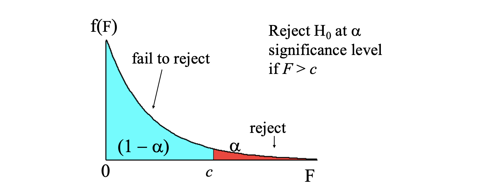
Test Hypotesis

Before starting with the test, let's take a look to the different errors:

Type I Error: we reject the null hypotesis when it is true (false positive).

α = P (H_{0} rejected when it is true)

Type II Error: we don't reject the null hypotesis when it is false (false negative).

β = P (failing to reject H_{0} when it is false)

$t$ Test

Set up the hypothesis. $H_{0}, H_{1}$ can be one-sided ( $H_{0} : b_{j} \leq 0, H_{1} : b_{j} > 0$ ) or two sided ( $H_{0} : b_{j} = 0, H_{1} : b_{j} \neq = 0$ ).
Determine the $t$ -statistic using the estimates for $b_{j}, se (b_{j})$ .

For example, as seen before: $t = \frac{b _{j} - 0}{se ( b _{j} )}$

Select a significance level, or, in other terms, the chance to make a Type I error and determine the critical value, depending if it is a one- or two-sided hypothesis.
Decide: reject $H_{0}$ if the absolute value of the $t$ -statistic is larger than the critical value.

For example, let's consider the following model:

employment = b_{0} + b_{1} education + ... + b_{k} x_{ik} + μ_{i}

We set up the hypotesis: $H_{0} : b_{1} \leq 0, H_{1} : b_{1} > 0$ ( $H_{0}$ : education doesn't increase employment)
We calculate $t = b_{1} / se (b_{1})$
We consider $c$ using $α$ (confidence level) and degree of freedom $= n - k - 1$
We reject $H_{0}$ if $t > c$ (if $H_{0} : b_{1} > 0$ use $t < - c$ )

If we reject the null hypotesis, we typically say: _ $x_{j}$ is statistically significant/has statistically significant effect on $y$ at the $α$ level.

Graphically:

Population Model

Quick summary remarks:

A coefficient is significant at the 5% level when its estimate is large relative to its standard error, equivalently when its absolute $t$ -statistic is large enough.
Do not confuse the size of an estimate with significance: a large effect can be imprecise, and a small effect can still be precisely estimated.
Significance answers a hypothesis-testing question; it does not by itself tell you whether the effect is economically important.
When a question asks for the number of significant coefficients, count the coefficients that reject the null individually, not the joint significance of the whole regression.
The intercept is tested exactly like any other coefficient, so include it unless the question explicitly excludes it.
If a coefficient is not significant, the safest interpretation is that the _ data do not provide enough evidence against the null at the chosen level._

More generally, we can test wheter an estimate fits a specific value: $H_{0} : b_{j} = a$ .

In this case, we use the appropriate $t$ -statistic: $t = (b_{j} - a) / se (b_{j})$ , where $a = 0$ for the standard test.

Confidence Intervals

Another way to use statistical testing is to construct confidence intervals using the same critical value for a two-sided test.

A $(1 - α) %$ confidence interval is defined as $b_{j} \pm c \cdot se (b_{j})$ where $c$ is the $(1 - α /2)$ percentile in a $t_{n - k - 1}$ distribution.

P-Values for $t$ -Tests

An alternative approach is to calculate what is the smallest significance level at which the null hypotesis would be rejected given the data.

So we compute the $t$ -statistic and we look up at which percentile it is in the appropriate $t$ -distribution. This is called the p-value.

The p-value represents the probability that we would observe the $t$ -statistic we did, if the null were true.

Testing more complex hypotheses - Linear Combination

Suppose we want to test if $b_{1}$ is equal to another parameter, that is: $H_{0} : b_{1} = b_{2}$ . Then the statistic test is $t = (b_{1} - b_{2}) / se (b_{1} - b_{2})$ .

But, if we expand the formula:

se (b_{1} - b_{2}) = Var (b_{1} - b_{2}) = Var (b_{1}) + Var (b_{2}) - 2 CoV (b_{1}, b_{2}) = = se (b_{1})^{2} + se (b_{2})^{2} - 2 s_{12}

So we need $s_{12}$ , which we don't usually have.

To avoid this, we can use the following "trick".

We set $H_{0} : q_{1} = b_{1} - b_{2} = 0$ . To do that, we also have to substitute $q_{1} = b_{1} - b_{2}$ in our model.

So, for example, we can consider:

y = b_{0} + b_{1} x_{1} + b_{2} x_{2} + μ ⟹ y = b_{0} + q_{1} x_{1} + b_{2} (x_{1} + x_{2}) + μ

Multiple Linear Restrictions

So far we tested a single linear restriction ( $b_{1} = 0, b_{1} = b_{2}$ ). Now we want to jointly test multiply hypotesis about the parameters.

A typical example is testing "exclusion restrictions", that means knowing if a group of parameters are equal to zero.

Then the null hypotesis might be something like: $H_{0} : b_{k - q + 1} = 0 = ... = b_{k} = 0$ , but we cannot check each statistic separately because we want to know fi the $q$ parameters are jointly significant each other.
We instead need to estimate:

the restricted model without all the $x_{k - q + 1} .. x_{k}$
the unrestricted model with all the $x$ included.

Intuition: we want to know if the change in SSR is bigh enough.

This is called the $F$ -statistic, defined as:

F = \frac{( SS R _{r} - SS R _{u r} ) / q}{SS R _{u r} / ( n - k - 1 )}

where $r$ is the restricted, $u r$ the unrestricted. Note that the $F$ statistic is always positive.

_Intuition: the $F$ statistic is measuring the relative increase in the SSR when moving from the unrestricted to the restricted model.

- $q = d f_{r} - d r_{u r}, d f_{u r} = n - k - 1$ .

To decide if the increases in SSR is "big enough", to reject the exclusions, we compare if with the $F$ distribution, indeed we know that: $F \sim F_{q, n - k - 1}$ where:

$q$ is the numerator degrees of freedom
$n - k - q$ is the denominator degrees od freedom.

f testl

OLS asymptotics

Under the Gauss-Markov assumptions the OLS is BLUE; however they are not always fulfilled with real data. Large samples (big data!) come to our rescue! It can be shown that some nice properties remain intact if $n \to \infty$ . (Larger samples allow us to relax some assumptions).

Consistency: if $n \to \infty$ estimators are consistent, that means that the distribution of the estimator collapses to the parameter value.
This implies that when $n \to \infty$ we can use MLR.4 (zero mean and zero correlation).

Just as we derived the omitted variable bias earlier, we can think about the inconsistency (asymptotic bias).

Consider the true model $y = β_{0} + β_{1} x_{1} + β_{2} x_{2} + v$ and the estimated model: $y = β_{0} + β_{1} x_{1} + μ$ , so that $μ = β_{2} x_{2} + v$ .
In this case, $b_{1} = β_{1} + β_{2} δ$ , where $δ = \frac{Cov ( x _{1} , x _{2} )}{Var ( x _{1} )}$ , which tells us how much our estimate ( $b_{1}$ ) deviates from the true parameter ( $β_{1}$ ).

Intuition: inconsistecy is a large sample problem: it does not go away as we add data.

Large Sample Inference

So far, we relied on assumption about normal distribution of errors, but this assumption can often break down! Again, large samples come to the rescue: as $n \to \infty$ , the central limit theorem shows that OLS estimates are asymptotically normal.

Thus, we no longer need to assume normality with a large sample, we get it anyway.

If $μ$ is not normally distributed, we sometimes will refer to the standard error as the asymptotic standard error. In general, we can expect standard errors to shrink at a rate proportional to the inverse of $n$ .

Asymptotic Efficiency

Thereare other estimators besided OLS that are consistent. However, under the Gauss-Markov assumptions, the OLS estimators will have the smallest asymptotic variances, therefore we say that the OLS is asymptotically efficient.

5 Multiple Regression Analysis: Further Issues

Review

To test hypotheses about estimates, we previously relied on assumption about normal distribution of errors (MLR.6) in order to redive $t$ and $F$ distributions.

This implied that the distribution of $y$ given $x$ was normal as well.

However, this assumption about normality can often break down! (example: a clearly skewed variable, like wages, arrests, savings etc., cannot be normal, since normal distributions are symmetric).

Also in this case, large samples are the solution: if $n \to \infty$ the Central Limit Theorem shows that OLS estimates are asymptotically normal.

In other terms, for any population with mean $μ$ and standard deviation $σ$ , the sampling distribution of the sample mean is approx normal with mean $μ$ and standard deviation $σ / n$ .

Secondly, the $t$ -distributoin approaches a normal distribution for a large $df$ (degree of freedom), so we no longer need to assume normality with a large sample.

As we said, if the error is NOT normally distributed, we sometimes will refer to it as the asymptotic standard error. (We can expect standard errors to shrink at rate proportional to the inverse of $n$ ).

Further Issues in Multiple Regression Analysis: Scaling Variables

Changing the scale of the $y$ variable will lead to a change in the scale of the coefficients and the standard error, without a meaningful change in significance/interpretation. The same applies for a change in $x$ .

Occasionally, we will see references to standardized coefficient, calculated using the standardized version of $x, y$ , so coefficients reflect a standard deviation change of $y, x$ .

Functional Form

OLS can also be used for relationship that are not strictly linear in $x, y$ by using non-linear functions of $x, y$ (as long the model is linear in the parameters).

Model	Equation	Interpretation
Level-level	$y = β_{0} + β_{1} x + u$	$Δ y = β_{1} Δ x$
Level-log	$y = β_{0} + β_{1} ln (x) + u$	$Δ y = (β_{1} /100)$
Log-level	$ln (y) = β_{0} + β_{1} x + u$
Log-log	$ln (y) = β_{0} + β_{1} ln (x) + u$

Log Models

they are invariant to the sale of the variables since it's all about percentage changes
they give a direct estimate of the elasticity
for models with $y > 0$ , the conditional distribution is often Heteroskedastic or skewed, whil $ln (y)$ is much less.
the distribution of $ln (y)$ is narrower, limiting the effect of outliers.

Note that, when using the log form, variables have to be positive!

Quadratic Models

For a model like $y = β_{1} x_{1} + β_{2} x_{2}^{2} + μ$ we know that:

if $β_{1}$ is positive and $β_{2}$ is negative, $y$ is increasing in $x$ at first and then decreasing.
if $β_{1}$ is negative and $β_{2}$ is positive the opposite happens.
The turning point is calculated setting the derivative to zero and lies at: $x^{*} = - β_{1} / β_{2}$

AdjustedR-Squared

Recall that $R^{2}$ always icrease as more variables are added to the model since $SSR$ never decreases with more variables:

R^{2} = \frac{SSE}{SST} = 1 - \frac{SSR}{SST}

The adjusted $R^{2}$ takes then into account the number of variables in the model:

Adj. R^{2} = 1 - \frac{SSR}{SST} \frac{( n - 1 )}{( n - k - 1 )}

The adjusted $R^{2}$ penalies models with more variables, especially for low $n$ and high $k$ and increases only when additional variables are added whose $t$ -statistic is larger than $\approx$ 1. $⟹$ adding variables with poor explanatory opower decreases adjusted $R^{2}$ .

In other terms, we usually use adjusted $R^{2}$ to compare models with the same $y$ , but never with models with different $y$ .

(Standard Errors for) Predictions

Suppose we want to use our estimates to obtain a specific prediction, in this case we want to estimate:

E (y ∣ x_{1} = c_{1}, ..., x_{k} =_{k}) = θ_{0} + b_{0} + b_{1} c_{1} + ... b_{k} c_{k}

If we want to have an idea of the precision of the estimate (easily done by substituting values) we can:

rewrite $β_{0} = θ_{0} - β_{1} c_{1} - ... β_{k} c_{k}$
substitute in to obtain: $y = θ_{0} + β_{1} (x_{1} - c_{1}) + ... + β_{k} (x_{k} - c_{k}) + μ$
regress $y_{i}$ on $(x_{ij} - c_{ij})$ and the intercept will gie the predicted value and its standard error $⟹$ the minum standard error is obtained when the $c$ equal the means of the $x$ .

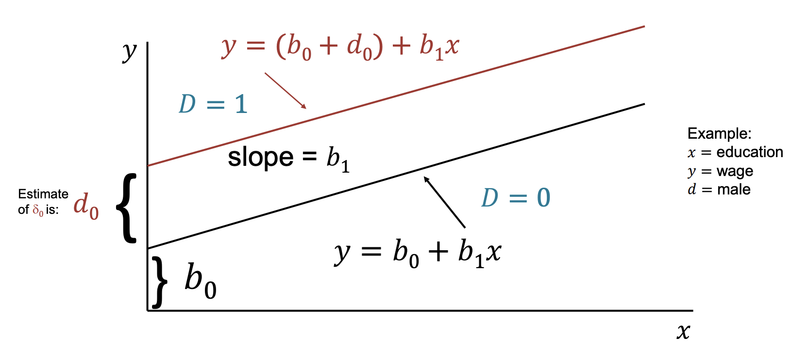
Regression with Dummy Variables

A dummy (binary) variable is variable that takes on the value of $1$ o $0$ .

Consider a simple model with one continuous variable $x$ and a dummy $D$ :

y = β_{0} + δ_{0} D + β_{1} x_{1} + μ

$D = 1$ if female, $0$ otherwise
$x$ : education in years
$y$ : wage

This can be interprete as an incercept shift:

if $D = 0 ⟹ y = β_{0} + β_{1} x_{1} + μ$ (male, BASE GROUP)
if $D = 1 ⟹ y = (β_{0} + δ_{0}) + β_{1} x_{1} + μ$ (female)

Population Model

Dummies for Multiple Categories

Any categorial variable can be turned into a set of dummy variables. Because the base group is represented by the intercept, if there are $n$ categories there should be $n - 1$ dummy variables.

Note that we can model interaction between dummies to divide in subgroups and between dummies with continuous variables $x$ to model a change in slope.

Dummy Vars

Testing for Differences Acorss Groups

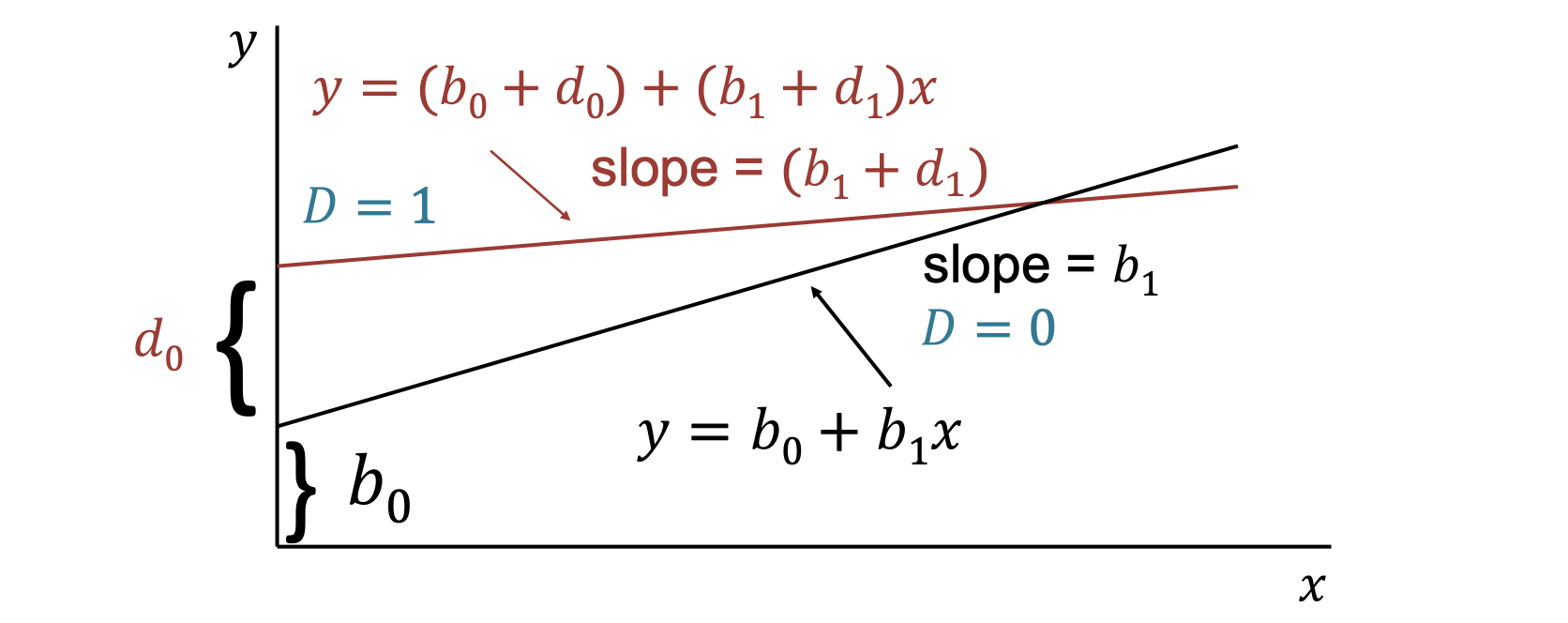
Testing wheter a regression function is different for one group versun one another can be thought as of testing for the joint significance of the dummy and its interaction with all other $x$ variables.

So we can estimate the model with and without the interactions and form a $F$ -statistic (very tedious in practise!).

The Chow Test

We can compute the $F$ -statistic without running the unrestricted model with all interactions with $k$ continuous variables, but intead we can:

run the restricted model for group 1 _(using observations $n_{1}$ ) and get $SS R_{1}$
run the restricted model for group 2 _(using observations $n_{2}$ ) and get $SS R_{2}$
run the restricted model for all _(using $N = n_{1} + n_{2}$ ) and get $SSR$
compute the $F$ -statistic as:

F = \frac{[ SSR - ( SS R _{1} + SS R _{2} )]}{SS R _{1} + SS R _{2}} \frac{n - 2 ( k + 1 )}{k + 1}

Dummy as Dependent Value: Linear Probability Model

$P (y = 1∣ x) = E [y ∣ x]$ when $y$ is binary model, so we can write our model as:

P (y = 1∣ x) = β_{0} + β_{1} x_{1} + ... + β_{k} x_{k} + μ

$β_{j}$ represents the change in the probability when $x_{j}$ changes by 1 around the mean.
the predicted $y$ is the probability

However, potential problems arise since the prediction can be outside $[0, 1]$ .
Also, this model will violate the assumption of homoskedasticity, which will affect inferece.

Despite everything, OLS is usually a good starting point when $y$ is binary.

6 Heteroskedasticity and Other Problems

Assumptions Multiple Linear Regressin (MLR) Model

MLR.1: Linear in parameters
- In the population model, the following relationship holds:

y = β_{0} + β_{1} x_{1} + \dots + β_{k} x_{k} + u

MLR.2: Random sampling
- We have a random sample of size $n$ :

{(y_{i}, x_{i 1}, \dots, x_{ik})}_{i = 1}^{n}

MLR.3: No perfect collinearity
- None of the independent variables is constant, and there are no exact linear relationships among regressors.
MLR.4: Zero conditional mean
- The error has zero conditional mean:

E [u ∣ x_{1}, x_{2}, \dots, x_{k}] = 0

This implies $E [u] = 0$ .
MLR.5: Homoskedasticity
- Assume constant conditional variance of the error:

Var (u ∣ x_{1}, x_{2}, \dots, x_{k}) = σ^{2}

MLR.6: Normality
- The disturbance is independent of $x_{1}, \dots, x_{k}$ and normally distributed with zero mean and variance $σ^{2}$ :

u \sim N (0, σ^{2})

Recall that the assumption of homoskedasticity implied that, conditional on the explanatory variables, the variance of the unobserved error $μ$ was costant.
If this is not true, then the variance is different for different values of $x$ and errors are said to be heteroskedastic.

Population Model

OLS is still unbiased and consistent, even if we do not assume homoskedasticity.

However, the standard errors of the estimates are biased if we have heteroskedasticity.

If the standard errors are biased, we cannot do inferece based on the usual $t$ , $F$ , $L M$ -statistic. (The $L M$ -statisitc is $L M : n R_{μ}^{2}$ , and $R_{μ}^{2}$ is obtained regressing $μ$ on all variables. The LM statistic has a $X_{k}^{2}$ -distributio.)

Variance with Heteroskedasticity

For the simple bivariate case, heteroskedasticity implies that:

OLS slope decomposition:

b_{1} = β_{1} + \frac{\sum _{i = 1}^{n} ( x _{i} - x ˉ ) u _{i}}{\sum _{i = 1}^{n} ( x _{i} - x ˉ ) ^{2}}

Conditional variance of $b_{1}$ under heteroskedasticity:

Var (b_{1} ∣ X) = \frac{\sum _{i = 1}^{n} ( x _{i} - x ˉ ) ^{2} σ _{i}^{2}}{( SS T _{x} ) ^{2}}, SS T_{x} = i = 1 \sum n (x_{i} - \overset{x}{ˉ})^{2}

Note that this differs from the homoskedastic case

Var (b_{1} ∣ X) = \frac{σ ^{2}}{SS T _{x}}

A valid (consistent) estimator of the variance of $b_{1}$ when $σ_{i}^{2} \neq = σ^{2}$ is:

Var (b_{1}) = \frac{\sum _{i = 1}^{n} ( x _{i} - x ˉ ) ^{2} u ^ _{i}^{2}}{( SS T _{x} ) ^{2}}

where $\overset{u}{^}_{i}$ are the OLS residuals.

Note that this is different from the homoskedastic estimator:

Var (b_{1}) = \frac{\frac{1}{n - 2} \sum _{i = 1}^{n} u ^ _{i}^{2}}{SS T _{x}} = \frac{SSR}{( n - 2 ) SS T _{x}}

Robust Standard Errors

Consider the model:

y = β_{0} + β_{1} x_{1} + \dots + β_{k} x_{k} + u

With heteroskedasticity, a valid (consistent) estimator of $Var (b_{j})$ is:

Var (b_{j}) = \frac{\sum _{i = 1}^{n} r _{ij}^{2} u ^ _{i}^{2}}{( SS R _{j} ) ^{2}}

where:

$r_{ij}$ is the $i$ -th residual from regressing $x_{j}$ on all other independent variables.
$SS R_{j} = \sum_{i = 1}^{n} r_{ij}^{2}$ is the sum of squared residuals from this auxiliary regression.
$\overset{u}{^}_{i}$ are the OLS residuals from the original model.

So, the corresponding robust standard error is:

se_{ro b} (b_{j}) = Var (b_{j})

Sometimes a finite-sample correction is used:

Var_{corr} (b_{j}) = \frac{n}{n - k - 1} Var (b_{j})

As $n \to \infty$ , this correction becomes negligible.

Note that robust standard errors are justified asymptotically. In small samples, $t$ -statistics based on robust SE may not be close to a $t$ distribution.

Testing for Heteroskedasticity

We want to test:

H_{0} = Var (μ ∣ x_{1}, ... x_{k}) = σ^{2} ⟺ H_{0} : E (μ^{2} ∣ x_{1}, ... x_{k}) = E = σ^{2}

If we assume the relationship betwee $μ^{2}$ and $x_{j}$ to be linear, we can test it as a linea restriction:

μ^{2} = δ_{0} + δ_{1} x_{1} + ... + δ_{k} x_{k} + v ⟺ H_{0} : δ_{1} = ... = δ_{k} = 0

The Breush-Pagan Test

In this test, we do not observe the error, but we can estimate it with the residuals from the OLS regrssion.

After regressing the residuals squared on all $x$ , we can use the $R^{2}$ to form a $F$ or $L M$ -test.

The $F$ -statistic is distributed as $F_{k, n - k - 1}$ and it is equal to:

F = \frac{R ^{2} ( n - k - 1 )}{( 1 - R ^{2} ) k}

THe $L M$ -statistic follows a $X_{k}^{2}$ -distribution and is:

L M = n R^{2}

Note that the Bresuch-Pagan test detect any linear forms of heteroskedasticity.

The White Test

The White Test allows for non-linearities by using squares and cross-products of all $x$ .

Consider thenm the fitted values from OLS $\overset{y}{^}$ are a function of all $x$ . Therefore $\overset{y}{^}^{2}$ will be a function of the squares and cross-produts, so we can:

regress the residuals squared on $\overset{y}{^}, \overset{y}{^}^{2}$
use the $R^{2}$ to form a $F$ or $L M$ -statistic

Weighted Least Squares

While it is always possible to estimate robust standard errors, if we know something about the specific form of heteroskedasticity we can obtain a more efficient estimates.

Intuition: transforming the model into one that has homoskedastic errors $⟹$ if we do it, we call the estimators weighted least squares.

Suppose the original model is: $y_{i} = β_{0} + β_{1} x_{i 1} + \dots + β_{k} x_{ik} + μ_{i}$

and heteroskedasticity has the form:

Var (μ_{i} ∣ x_{i}) = σ^{2} h_{i}, h_{i} = h (x_{i}) > 0

We can define the variable:

μ_{i}^{*} = \frac{μ _{i}}{h _{i}}

Because $h_{i}$ is a function of $x_{i}$ , conditional on $x_{i}$ it is a constant and has costant variance.

E (μ_{i}^{*} ∣ x_{i}) = E (\frac{μ _{i}}{h _{i}} x_{i}) = \frac{1}{h _{i}} E (μ_{i} ∣ x_{i}) = 0

Var (μ_{i}^{*} ∣ x_{i}) = Var (\frac{μ _{i}}{h _{i}} x_{i}) = \frac{1}{h _{i}} Var (μ_{i} ∣ x_{i}) = \frac{1}{h _{i}} σ^{2} h_{i} = σ^{2}

Hence the transformed error is homoskedastic.

We now trasform the whole equation model by dividing the original model by by $h_{i}$ :

\frac{y _{i}}{h _{i}} = β_{0} \frac{1}{h _{i}} + β_{1} \frac{x _{i 1}}{h _{i}} + \dots + β_{k} \frac{x _{ik}}{h _{i}} + \frac{μ _{i}}{h _{i}}

We can then define the transformed variables as:

y_{i}^{*} = \frac{y _{i}}{h _{i}}, x_{ij}^{*} = \frac{x _{ij}}{h _{i}}, c_{i} = \frac{1}{h _{i}}, u_{i}^{*} = \frac{μ _{i}}{h _{i}}

so we obtain:

y_{i}^{*} = β_{0} c_{i} + β_{1} x_{i 1}^{*} + \dots + β_{k} x_{ik}^{*} + u_{i}^{*}

E (u_{i}^{*} ∣ x_{i}) = 0, Var (u_{i}^{*} ∣ x_{i}) = σ^{2}

So OLS on this transformed model is BLUE (under the usual assumptions).

But why this is called “weighted” least squares?

OLS on transformed data minimizes:

i = 1 \sum n (y_{i}^{*} - β_{0} c_{i} - j = 1 \sum k β_{j} x_{ij}^{*})^{2} = i = 1 \sum n \frac{( y _{i} - β _{0} - \sum _{j = 1}^{k} β _{j} x _{ij} ) ^{2}}{h _{i}} = i = 1 \sum n \frac{u ^ _{i}^{2}}{h _{i}}

Therefore WLS minimizes weighted residual squares with weights $w_{i} = \frac{1}{h _{i}}$

Intuition:

If $h_{i}$ is large, observation $i$ has high error variance $\Rightarrow$ lower weight.
If $h_{i}$ is small, observation $i$ has low error variance $\Rightarrow$ higher weight.

Feasible GLS (FGLS) for Unknown Heteroskedasticity

In reality, we often do NOT know the exact form of heteroskedasticity ( $h (x)$ ), so we need to estimate it.

We generally assume a flexible variance model:

Var (u_{i} ∣ x_{i}) = σ^{2} exp (δ_{0} + δ_{1} x_{i 1} + \dots + δ_{k} x_{ik})

So, under this assumption, we have:

Var (u_{i} ∣ x_{i}) = σ^{2} h (x_{i}), h (x_{i}) = exp (δ_{0} + δ_{1} x_{i 1} + \dots + δ_{k} x_{ik})

Note that exponential form guarantees $h (x_{i}) > 0$ , so variance cannot be negative.

From this assumption:

u_{i}^{2} = σ^{2} exp (δ_{0} + δ_{1} x_{i 1} + \dots + δ_{k} x_{ik}) v_{i}

if we assume $v_{i}$ independent of $x_{i}$ and

E (v_{i} ∣ x_{i}) = 1

If we take the logarithms we obtain:

ln (u_{i}^{2}) = α_{0} + δ_{1} x_{i 1} + \dots + δ_{k} x_{ik} + e_{i}

α_{0} = ln (σ^{2}) + δ_{0}, e_{i} = ln (v_{i}), E (e_{i} ∣ x_{i}) = 0

Since $u_{i}$ is unobserved, use OLS residuals $\overset{u}{^}_{i}$ from the original regression and estimate:

ln (\overset{u}{^}_{i}^{2}) = α_{0} + δ_{1} x_{i 1} + \dots + δ_{k} x_{ik} + e_{i}

Let fitted values from this auxiliary regression be $\overset{g}{^}_{i}$ , then:

\hat{h}_{i} = exp (\overset{g}{^}_{i})

with weights equals $w_{i} = \frac{1}{h ^ _{i}}$ .

Specification and Data Issues

We have seen that a linear regression can really fit nonlinear relationship, but how do we know if we have the right functional form for our model?
Firstly, economic theory shoud guide you, but a test of functional form can be useful.

Ramsey's RESET (Regression Specification Error Test)

RESET test lies on a trick similar to the special form of the White Test.

Instead of adding functions of the $x$ directly, we add and test functions on $\overset{y}{^}$ :

estimate $y = β_{0} + β_{1} x_{1} + ... + β_{k} x_{k} + δ_{1} \overset{y}{^}^{2} + δ_{2} \overset{y}{^}^{3} + v$
test: $H_{0} : δ_{1} = δ_{2} = 0$
a significant $F$ -test suggests that the model is not correctly specified _(using $F \sim F_{2, n - k - 3}$ or $L M \sim X_{k}^{2}$ )

What the test does: the RESET adds nonlinear (and/or interaction) functions of the fitted values $\overset{y}{^}$ to the regression to detect whether important non-linearities or omitted transformations are missing from the specified model form. Under the null hypothesis the added coefficients (here $δ_{1}$ , $δ_{2}$ ) are zero, so the restricted model (original regression) is OK with respect to them.

How to read the F-statistic:

Degrees of freedom: numerator $q =$ number of added terms (2 here); denominator = $n - K - q$ , where $K$ is the number of parameters estimated in the original model (including the intercept). The test compares the restricted SSR to the unrestricted SSR.
Decision rule: compute the F-statistic and either compare it to the critical value from $F_{q, n - K - q}$ at the chosen $α$ or use the p-value. If $F > F_{cr i t}$ or $p < α$ , reject $H_{0}$ and conclude there is evidence the model is misspecified.

Practical interpretation and next steps: a significant RESET does not tell you which specific variable or transformation is missing — only that the current functional form is likely inadequate. After rejection, examine residual plots, try theory-driven transformations (logs, polynomials, interactions), include specific nonlinear terms of $x$ (rather than $\overset{y}{^}$ powers alone), or run targeted specification tests. If the RESET is not significant you have no evidence (from this test) of the particular misspecifications it detects, but this is not proof the model is correct.

Proxy Variables

What if a model is mis-specified because no data is available on a important $z$ variable?

It's possible to avoid omitted variable bias using a proxy variable. A proxy variable must be related to the unbobservable variable.

Consider for example: $y = β_{0} + β_{1} x_{1} + β_{2} x_{2} + β_{3} x_{3} + μ$ and suppose we do NOT have data about $x_{3}$ but we have data on other inputs, so we can write:

x_{3}^{*} = δ_{0} + δ_{3} \overset{x}{^}_{3} + v_{3}

where $*$ implies unobserved. Then we can just substitute $x_{3}$ for $x_{3}^{*}$ .

However, to have consistent estimates of $β_{1}, β_{2}$ , we need:

E (x_{3}^{*} ∣ x_{1}, x_{2}, x_{3}) = x_{3}^{*} ∣ x_{3} = δ_{0} + δ_{3} x_{3}

or, in other terms, we need $μ$ uncorrelated with $x_{1}, x_{2}, x_{3}^{*}$ and $v_{3}$ uncorrelated with $x_{1}, x_{2}, x_{3}$ .

Only in this case we can run the regression:

y = (β_{0} + β_{3} δ_{0}) + β_{1} x_{1} + β_{2} x_{2} + β_{3} x_{3} + (μ + β_{3} v_{3})

Without the previous assumption, we could end up with biased estimates:

If we consider for example $x_{3}^{*}$ correlated with $x_{1}, x_{2}, x_{3}$ :

x_{3} = δ_{0} + δ_{1} x_{1} + δ_{2} x_{2} + δ_{3} x_{2} + v_{3}

them we end up in the regression:

y = (β_{0} + β_{3} δ_{0}) + (β_{1} + β_{3} δ_{1}) x_{1} + (β_{2} + β_{3} δ_{2}) x_{2} + β_{3} δ_{3} x_{3} + (μ + β_{3} v_{3})

Intuition: the bias depends on the signs of $β_{3}, δ_{j}$ , but it is still smaller than the omitted variable bias.

Measurement Error in a dependent variable

Consider the following situation. We would like to esitimate: $y^{*} = β_{0} + β_{1} x_{1} + ... β_{k} x_{k} + μ$ but we only measure the true value plus an error:

y = y^{*} + e_{0}

We then define the measurement error $e_{0} = y - y^{*}$ .

Therefore, we really estimate:

y = β_{0} + β_{1} x_{1} + ... β_{k} x_{k} + μ + e_{0}

if $e_{0}$ and $x_{j}$ are uncorrelated, then the estimate is unbiased
if $E [e_{0}] = 0$ , then the estimate of $β_{0}$ is biased

Measurement Error in an Explanatory Variable

We want to estimate: $y = β_{0} + β_{1} x_{1}^{*} + μ$ , so we define the measurement error as $e_{1} = x_{1} - x_{1}^{*}$ and we assume:

E [e_{1}] = 0, E [y ∣ x_{1}^{*}, x_{1}] = E [y ∣ x_{1}^{*}]

Therefore, we really estimate:

y = β_{0} + β_{1} x_{1} + (μ - β_{1} e_{1})

The effect of the measurement error depends on assumptions abou the correlation betweeen $e_{1}, x_{1}$ :

if $Cov (x_{1}, e_{1}) = 0$ : OLS remains unbiased but we get higher variaces (similar to the proxy variable case)
if $Cov (x_{1}^{*}, e_{1}) = 0$ _(case known as the Classical errors-in-variavles assumption) $⟹ x_{1}, e_{1}$ are correlated with:

Cov (e_{1}, x_{1}) = E [x_{1} e_{1}] = x_{1}^{*}, e_{1} + E [e_{1}^{2}] = 0 + σ^{2}

This implies that $x_{1}$ is correlated with the error so the estimate is biased:

n \to \infty lim (b_{1}) = β_{1} + \frac{Cov ( x _{1} , μ - β _{1} e _{1} )}{Var ( x _{1} )} = = β_{1} + \frac{β _{1} σ _{e}^{2}}{σ _{x}^{2} + σ _{e}^{2}} = β_{1} + \frac{β _{1} σ _{x^{*}}^{2}}{σ _{x}^{2} + σ _{e}^{2}}

Note that the multiplicative error is $< 1$ so the estimate is biased toward zero (attenuatoin bias).

Nonrandom Samples

If the sample is chosen on the basis of an $x$ variable, then estimates are unbiased.

If the sample is chosen on the basis of the $y$ variable, them we sample selection bias.

Note that sample selection can be very subtle! For example, looking at wages for workers (people choose to work for this wage) is different that looking for the wage offers.

Outliers

Sometimes an individual observation can be very different from the others and can have large effects on the outcome. Outliers are often caused by errors in data entry (reason why looking at data summary statistic is very important!).

Multiple strategies to deal with outliers:

fix observation where it is clea there was just an extra zero or similar
drop outlier observations and show regressions with/without them
winsorize estreme observations (for istance: observations below $p 1$ set to $p 1$ and above $p 99$ set to $p 9$ ).

7 Time Series Data

Time sereis data have a temporal ordering:

y_{t} = β_{0} + β_{1} x_{1} + μ_{t}

Recall that, on the other hand, cross sectional data : $y_{i} = β_{0} + β_{1} x_{i} + μ_{i}$ .

So, instead of having a random sample of individuals, we have one realization of a stochastic process, therefore we need to adapt some assumptions for OLS.

Examples of Time Series Models

A static model related contemporaneous variables:

y_{t} = β_{0} + β_{1} z_{t} + μ_{t}

A finite distributed lag (FDL) model with otder $n$ (in which we then have $n$ lags) allows one or more variables to affect $y$ with a lag:

y_{t} = α_{0} + δ_{0} z_{t} + δ_{1} z_{t - 1} + ... + δ_{n} z_{t - n} + μ_{t}

We call $δ_{0}$ the impact propensity that reflects the immediate change in $y$ given by $z$ .
$δ_{i}$ represent the change in $y$ $i$ periods after a one-period change in $z$ . (so for a temporary 1 period change in $z$ , $y$ returns to its original level in $n + 1$ periods).
We call $δ_{0} + ... + δ_{n}$ the long-run propensity (LRP) that reflects the long-run change in $y$ after a permanent change in $z$ .

Properties

We now take some time to understand which properties need to be adapted to time series data in order to use OLS in a proper way. Recall that the MLR assumptions are (as discussed before):

MLR.1: Linear in parameters: $y_{i} = β_{0} + β_{1} x_{i 1} + \dots + β_{k} x_{ik} + u_{i}$
MLR.2: Random sampling
MLR.3: No perfect collinearity
MLR.4: Zero conditional mean: $E (u_{i} ∣ x_{i 1}, x_{i 2}, \dots, x_{ik}) = E (u_{i}) = 0$
MLR.5: Homoskedasticity: $Var (u_{i} ∣ x_{i 1}, x_{i 2}, \dots, x_{ik}) = σ^{2}$
MLR.6: Normality

Recall also that:

MLR.1 to MLR.5 $⟹$ OLS is unbiased and BLUE
MLR.% $⟹$ we can do inference (hypotesis testing) in small samples.

In order to still have a unbiased OLS, for time series data we need the following properties:

TS.1: Linear in parameters
- The stochastic process ${(x_{t 1}, \dots, x_{t k}, y_{t}) : t = 1, \dots, n}$ follows the linear model:
$y_{t} = β_{0} + β_{1} x_{t 1} + \dots + β_{k} x_{t k} + u_{t}$
TS.2: No perfect collinearity
- In the sample, no independent variable is constant and no independent variable is a perfect linear combination of the others.

TS.3: Zero conditional mean $E (u_{t} ∣ X) = 0, t = 1, \dots, n$
- where $x_{t} = (x_{t 1}, \dots, x_{t k})$ and $X$ collects all explanatory variables for all time periods.
- Implication: the error term in any given period is uncorrelated with explanatory variables in all periods (regressors are strictly exogenous).

Alternative assumption (weaker) $E (u_{t} ∣ x_{t}) = 0$
- This implies regressors are contemporaneously exogenous.
- Contemporaneous exogeneity is generally sufficient for consistency in large samples.

Note that we skipped the assumption of a random sample:

the key impact of the random samples is that $μ_{i}$ is independent since the exogeinity assumption takes are of it in this case.
Based on these 3 assumptions, the OLS estimators are unbiased.
TS.3 can easily break down. If we consider for example $y_{t} = β_{0} + β_{1} x_{t 1} + μ_{t}$ when past value of $x$ affect $y$ but we just set up a contemporaneous model.

Variances of OLS estimators for Time Series Data

To derive variances of estimators, we stard with some assumptions. We then assume that the variance is independent of all the $x$ 's and it is costant over time (TS.4):

Var (μ_{t} ∣ X) = Var (μ_{t}) = σ^{2}

We also assume no-serial correlation: (TS.%)

Cor (u_{t}, μ_{s} ∣ X) = 0 \forall t \neq = s

Under TS.1 to TS.5 (Gauss-Markov Assumptions) the OLS variances in the time-series case are the same as in the cross-sectoin case, consequently we have:

the estimator of $σ^{2}$ is the same
OLS is BLUE.

With the additional inference (TS.6) of Normality (errors are independent of $X$ and are independently and identically distributed as Normal $μ_{t} \sim N (0, σ^{2})$ ):

inference is the same as before.

Comparison of the assumptions

Cross-section data	Time-series data
MLR.1: Linear in parameters; $y_{i} = β_{0} + β_{1} x_{i 1} + \dots + β_{k} x_{ik} + u_{i}$	TS.1: Linear in parameters; $y_{t} = β_{0} + β_{1} x_{t 1} + \dots + β_{k} x_{t k} + u_{t}$
MLR.2: Random sampling	No direct counterpart (time series are ordered in time, not randomly sampled)
MLR.3: No perfect collinearity	TS.2: No perfect collinearity
MLR.4: Zero conditional mean; $E (u_{i} ∣ x_{i 1}, x_{i 2}, \dots, x_{ik}) = 0$	TS.3: Zero conditional mean; $E (u_{t} ∣ X) = 0$
MLR.5: Homoskedasticity; $Var (u_{i} ∣ x_{i 1}, x_{i 2}, \dots, x_{ik}) = σ^{2}$	TS.4: Homoskedasticity; $Var (u_{t} ∣ X) = σ^{2}$
No serial-correlation assumption in cross-sectional baseline	TS.5: No serial correlation; $Cor (u_{t}, u_{s} ∣ X) = 0 for t \neq = s$
MLR.6: Normality	TS.6: Normality

Trending

Some examples of trend:

linear trend: $y_{t} = α_{0} + α_{1} t + e_{t}$
exponential trend: $lo g (y_{t}) + α_{0} + α_{1} t + e_{t}$
quadratic trend: $y_{t} = α_{0} + α_{1} t + α_{2} t^{2} + e_{t}$

Regression with a linear trend is the same things as using a "detrended" sereis in a regression.

Detrending implies regressing each variable on $t$ (including a costant) and than take the residuals of this regression (the result is the detrended series).

Some advaantages od detrending for calculating $R^{2}$ :

time-series regression tend to have a very high $R^{2}$ as the trend is "very well explained".
$R^{2}$ from a regression on detrended data better reflect how well $x$ explain $y$ .

Seasonality

Often time-series data has some periodicity, in this case there are two major practices:

adding a set of seasonal dummy variables
series can be ajusted before running the regression.

8 Panel Data

Pooled cross sectional data refer to data on individuals and periods where individuals cannot be followed explicitily over time (independent sampled observatoins with knowledge about the time dimension)
Panel data follow the same cross-sectional units over time.

Population Model

WHy should we use pooled cross-sections?

to get a bigger sample size and then more degrees of freedom for a more precise estimate
to investigate if the relations evolve over time
- Chow test: test if parameters change over time
to have more dimensions of variation: cross-section and time (difference in difference estimation, especially useful for evaluating policies)
- Example: do house prices at different locations change differently after a climate policy?

The Chow Test

It tests if there is difference in the slopes across 2 groups.

Basic idea: it's very similar to having 2 time periods as "groups" using a dummy variable for one of the two periods and test for joint significance of period (1) dummy and the period (2) interaction terms.

If we have multiple periods, we can do the following:

computer a proper $F$ statistic by running the strcited model allowing for dofferent time intercepts but no interaction with all the $k$ variables $⟹$ obtain $SSR_{r}$ .
run the restricted model for period one and get $SS R_{1}$ , then for period 2 etc etc....
they all form the unrestricted $SSR_{u} = \sum_{k} SSR_{k}$
then compute $F$ in the case of a twop period as:

F = \frac{\text{SSR}-(\text{SSR_1}+\text{SSR_2})}{\text{SSR_1}+\text{SSR_2}} \frac{n - 2(k+1)}{k+1}

The Chow test is just a simple $F$ test for exclusion/restriction.

note that we have $k + 1$ restrictions
note that the unrestricted model would estimate 2 different intercepts and slope coefficients, so the degree of freedom is $n - 2 (k + 1) = n - 2 k - 2$ .

In real-world economics, we can't run randomized experiments (RCTs) for ethical/practical reasons. We can just observe people's choices, which creates endogeneity (people self-select into treatments).

However, having repeated cross sections allows observing groups random samples of observations across time in data. Often policites can affect different groups differently, leaving a "trace" of variation that is sometimes "as good as randomly assigned" across groups.
We call such events natural experiments because they create an experimental setup with:

treatment group: the one assigned to treatment and trated after the event happened (but not before)
control group: the one that does not get treated and has not been treated before.

(Note that the timing and the assignment are outside of anyone's control)

Example: Minimum Wage & Employment (Card and Krueger, 1994)

This analysis focused on the New Jersey raising its minimum wage from $4.25 t o$ 5.05 per hour on April 1, 1992. Pennsylvania did not.

treatment group: fast-food workers in NJ (subjected to the wage increase)
control group: fast-food workers in Pennsylvania (no wage change, very close so similar market conditions)

Then the study analyzed the change in employment in the two states, finding that employment in NJ fast food actually increased slightly, in contrast to the traditional economic theory, suggesting that the minimum wage didn't reduce jobs.

Difference-in-Difference

Assume we have an experiment where units are randomly assigned to a treatment (A) and a control (B) group.

To estimate the treatment effect we compare the changes in outcomes from before and after the treatments and across two groups:

(\overset{y}{ˉ}_{A 2} - \overset{y}{ˉ}_{A 1}) - (\overset{y}{ˉ}_{B 2} - \overset{y}{ˉ}_{B 1}) = (\overset{y}{ˉ}_{A 2} - \overset{y}{ˉ}_{B 2}) - (\overset{y}{ˉ}_{A 1} - \overset{y}{ˉ}_{B 1})

and we label this as the Difference-in-difference (DiD) estimator in the group means.

We can then use a regression framework with dummy variables to do the same:

y_{i t} = β_{0} + β_{1} treatment_{i} + β_{2} after_{t} + β_{3} treatment_{i} \cdot after_{t} + μ_{t}

where:

$β_{0}$ : Baseline outcome (control group, before treatment)
$β_{1}$ : Pre-existing difference between treatment and control (should be $\approx 0$ if randomized)
$β_{2}$ : Time effect for the control group (secular trend unaffected by treatment)
$β_{3}$ : Difference-in-difference estimator (the additional change in the treatment group beyond the secular trend)

(Note that this model can be generalized with different dummies and interaction terms for different years)

Using the regression framework furthermore:

we can produce confidence intervals and to hypotesis testing
we can add additional variables to control the differences across the treatment and control group.

However, the DiD estimator could be biased:

if there are already existing ttrend prior to a policy. In this case, we should get more than 2 periods and show how groups follow different trends prior to the event.
if the grouos are affected by other policites/evets at the time time, in this case we should control for some other factors
spill-pover for treatment to control groups, in this case simply take a suitable control group that doesn't deviate
no selection bias if individuals cannot decide which group they are in

Advantage of using (real) Panel Data

With panel data, unlike pooled cross-sections, we can address the omitted variable bias caused by time-invariant individual-specific factors.

Suppose the population model is:

y_{i t} = β_{0} + β_{1} x_{i t 1} + ... + β_{k} x_{i t k} + a_{i} + μ_{i t}

where $a_{i}$ is the unobserved effect that is specific to the individual and does not vary over time. This forms a composite error: $v_{i t} = a_{i} + μ_{i t}$ .

If $a_{i}$ is correlated with the $x_{i t} ⟹$ OLS is biased and inconsistent (since we treated $a_{i}$ as part of the error term without explicitly controlling for it).

We can adopt three approaches to address these time-invariant unobserved effects:

First-difference (FD) estimator: take the first-difference of the equation, which removes both $a_{i}$ and $β_{0}$
Fixed-effect (FE) estimator: subtract the individual averages of all variables (demeaning), which removes both $a_{i}$ and $β_{0}$
Random-effect (RE) estimator: assume that $x_{i t}$ and $a_{i}$ are uncorrelated (can use all the data more efficiently, but is biased if this assumption fails)

First-difference Estimator

We perform $y_{i t} - y_{i t - 1}$ to obtain:

Δ y_{i t} = y_{i t} - y_{i t - 1} = β_{1} x_{i t - 1} + ... + β_{k} Δ x_{i t k} + Δ μ_{i t}

to estimate this with OLS, we need that each $De lt a x_{i t}$ is uncorrelated with $Δ_{u i t}$ , that only holfd if the $μ_{i t}$ is uncorrelated with each explanatory variable during the entire time sample
we need to assume strict exogeneity, $E [Δ μ_{i t} ∣Δ X_{j}, a_{j}] = 0$ .
this can be done for more that just two time periods when $T > 2$ .

However, note that when there's little variatin in the $Δ_{i t}$ standard errors will be large.

Fixed-effect Estimator

We then consider the individual mean with $a_{i} = 0, \overset{u}{ˉ}_{i} = 0$ :

\overset{y}{ˉ}_{i} = β_{0} + β_{1} \overset{x}{ˉ}_{i 1} + .... + β_{k} \overset{x}{ˉ}_{i l} + \overset{a}{ˉ}_{i} + \overset{μ}{ˉ}_{i}

and we opbtain the new model where $\overset{x}{¨}_{i t} = x_{i t} - \overset{x}{ˉ}_{i}$ :

\overset{y}{¨}_{i t} = y_{i t} - \overset{y}{ˉ}_{i t} = β_{1} \overset{x}{¨}_{i t 1} + ... + β_{k} \overset{x}{¨}_{i t k} + μ_{i t}

this is identical to including a separate incercept (dummy) for each individual $i$
we still need the strict exogeneity assumption
in this case we loose $N$ (number of individuals) degrees of freedom by de-meaning and we have to make sure that OLS uses $N (T - 1) - k$ degree of freedom.

If we compare the two previous models, we see that the main difference lies in the "no serial correlation assumption".

first-difference estimator's advantages is that unit root problems are solved
fixed effect is more efficient when $u_{i t}$ is serially correlated

Random Effect

Previously we assume that $a_{i}$ was correlated with the $x$ . If it is not the case, OLS would be consistent, but the composite error $v_{i t} = a_{i} + μ_{i t}$ would be serially correlated.

In this case, we can use the Generalized Least Squares (GLS) approach and trasform the model to make errors serially uncorrelated.

We start by doing:

θ = 1 - σ_{μ}^{2} / (σ_{μ}^{2} + T σ_{a}^{2})

then we subtract:

\theta \bar y_i = \beta_0 \theta + \beta_1 \theta \bar x_{i1} + ... + beta_k \theta \bar_{ik} + \theta \bar v_i

to obtain the new model:

\tilde y_{it} = \beta_1 \tilde x_{it} + ... + \beta_k \tilde x_{ik} + \tilde v_{it}, \quad \tilde_{it} = z_{it}- \theta \bar z_i

we end up with a sort of weighted averaged of OLS and fixed effects.

if $θ = 1 ⟹$ this is just the fixed effect estimator
if $θ = 0 ⟹$ this is just the OLS

also, the bigger the variance on the unobserved effect $σ_{a}^{2}$ , the closer is to FE, the smaller the variance, the closer to OLS.

Usually, iti is often more appropriate to use the fixed effect since the unobserved fixed effects are often correlated with the $x$ .

The testing procedure is the following:

Hausman Test (to compare fixed effects with random effects model):
- compare estimates of the $β$ -vector with and without the additional randome effect assumption
- if the additional assumptions are true, then the estimates should be similar.

Correlated Random Effects approach

We can end up in the case of $a_{i}$ split up between a part related to the time-averages of the explanatory variables and a part $r_{i}$ uncorrelaed to the explanatory variables.

a_{i} = α + t_{i} \overset{x}{ˉ}_{i 1} + ... + y_{k} \overset{x}{ˉ}_{k 1} + r_{i}

The resulting model is an ordinary random effects model with uncorrelaed random effect $r_{i}$ but with the time averages as additional regressors:

y_{i t} = (β_{0} + α) + β_{1} x_{i t 1} + ... + β_{k} x_{ik} + y_{1} + \overset{x}{ˉ}_{i 1} + ... y_{k} \overset{x}{ˉ}_{k 1} + (r_{i} + μ_{i t})

_Note that in this case the $β$ -vector is identical to the one of the fixed effect estimator.

We can also test the ordinary FE with the Corrrelated Random Effect approach, testing for the relevance of the $y$ -parameters (Mundlak Test)

9 Instrumental Variables

One of the most problematic assumption of OLS is the zero conditional meanassuption (the explanatory variables are assumed exogenous) $⟹$ it this doesn't hold, the parameter estimates are biaed and inconsistent.

So if the error term contains variables (i.e. if the error term is correlated with them) that are correlated with one of the explanatory variables we can:

pull the variable out of the error term including more relevant regressors
in case of panel data, assume that the variable is costant over time.

We consider then an example of regression with endogeneity problems: i.e. $Cov (x, μ) \neq = 0$ :

lo g wage_{i} = β_{0} + β educ_{i} + μ_{i}

and we know that $μ$ contains abilitiy, so $Cov (educ_{i}, μ) \neq = 0$ , so we if we use OLS, $β_{1}$ is biased and inconsistent due to omission of ability.

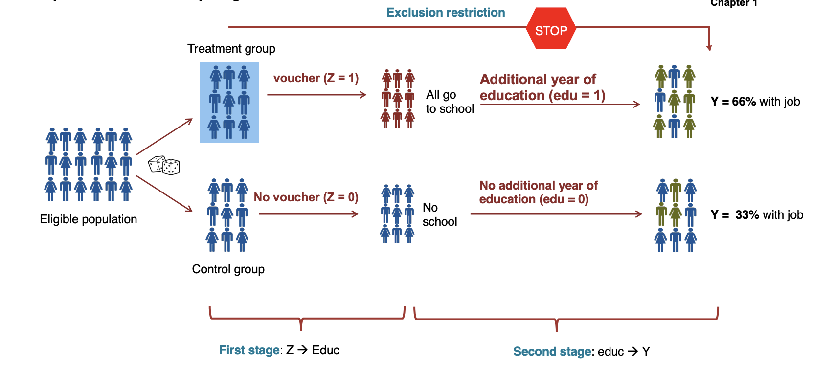
To solve this endogenity problem we use an instrumental variable (IV) denotes as $Z$ that:

is correlated with the endogenous variable
is uncorrelated with the error term $μ$
affects the dependent variable only through the endogenous variable (only by changing $X$ )

In the previous example:

$Z$ affects the number of years of education, so wehave $X = educ$
$Z$ indirectly affects wages $Y$ through its effect on education.

Conditions for valid instruments:

First Stage: $Cov (Z, X) \neq = 0$ ( $Z$ must be correlated with $X$ )
Independence: $Cov (Z, μ) = 0$ (the instrument must be endogenous)
Exclusion restriction: Z can affect the outcome only by changing $X$

Instrumental Variable

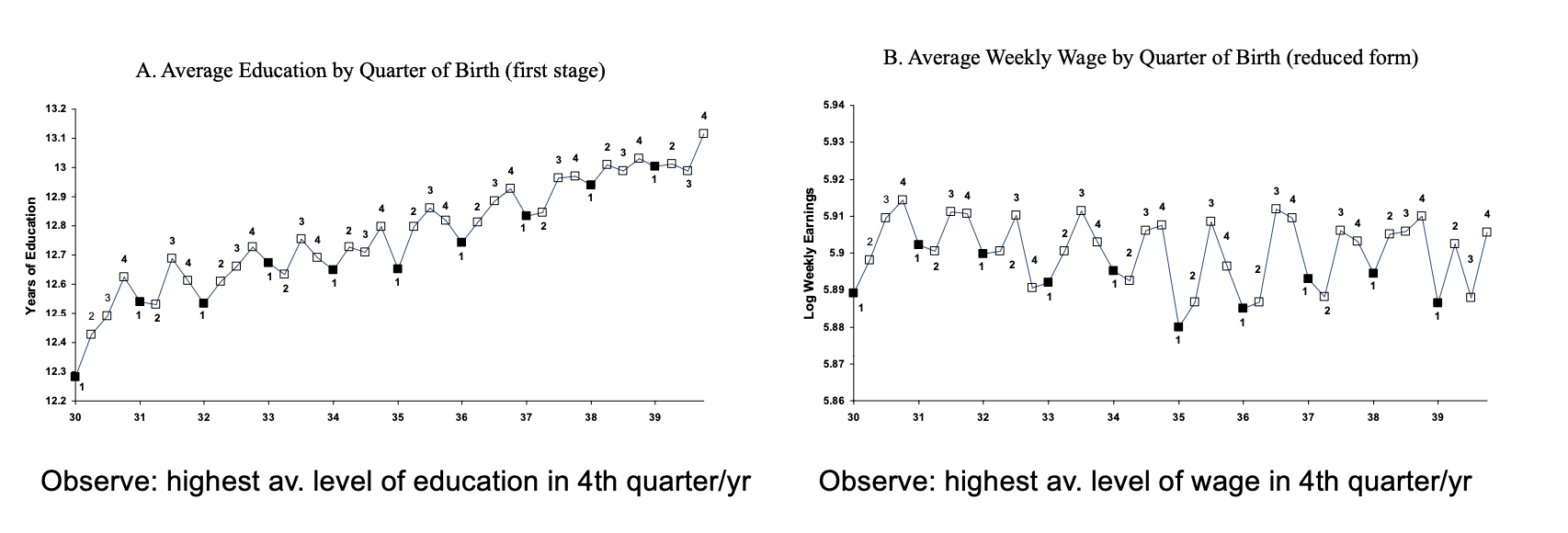
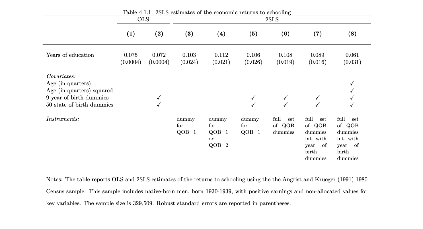
The Angrist and Krueger (1991) natural experiment (Nobel Prize 2021)

Angrist and Krueer studied which factors drive out of the full control of individuals (uncorrelated wth $μ$ ) drive education, finding an interesting variation created by US schooling laws in the early 1930:

Law 1: students enter school in calendar year in which they turn 6 $⟹$

School Starting Age = f (Date of birth)

Law 2: Compulsory schooling require students to remain in school until became $16$ so, since school starts for everyone in the same day of the month, depending on the birth date students can stay in school morel/less time.

So these laws can create a natural experiment that incluences the number of years of education.

In particular, they observed that, on average, people with born in the 4th quarter showed an higher average level of education.

Education = π_{10} + π_{11} Q4 + v_{1}

As a consequence, people born in the 4th quarter show higher average level of wage:

lo g (wage) = π_{20} + π_{21} Q4 + v_{2}

Instrumental Variable

Instrumental Variable Estiation in the Simple Regressoin Case

We consider the model with $x$ explanatory variable correlated with the error and $z$ instrumental variable (uncorrelated with $μ$ , correlated with $x$ ):

y = β_{0} + β_{1} x + μ

We firstly write the covariance of $x, y$ :

Cov (z, y) = Cov (z, β_{0} + β_{1} x + μ)

using the linerarity of covariance and that $Cov (z, μ) = 0$ , we then get:

Cov (z, y) = β_{1} Cov (z, x) + Cov (z, μ) ⟹ β_{1} = \frac{Cov ( z , y )}{Cov ( z , x )} ⟹ β_{1} = \frac{\frac{Cov ( z , y )}{Var ( z )}}{\frac{Cov ( z , x )}{Var ( z )}}

Them the IV estimator for $β_{1}$ is:

β_{1} = \frac{\sum ( z _{i} - z ^{a vg} ) ( y _{i} - y ^{a vg} )}{\sum ( z _{i} - z ^{a vg} ) ( x _{i} - x ^{a vg} )}

Two Stage Least Squares

IV estimation can be extended to the multiple instruments case. In this case we talk about Two Stage Least Squares (2SLS)

We consider the initial structural model (the equation we want to estimate, example):

lo g (wage) = b_{0} + b_{1} \cdot educ + b_{2} \cdot X + u

The goal is to estimate $b_{1}$ (the causal effect of educatoin on wages) while controlling for $X$ .

We are now assuming that both $z_{1}, z_{2}$ are valid instruments (correlated with $educ$ and uncorrelated with the error).
Note that $educ$ is the endogenous variable and $X$ are again exogenous regressors.

Stage 1: the best instrument is a linear combination of all the exogenous variables: so we regress the endogenous variable $educ$ on the instruments ( $Q 3, Q 4$ )and $X$ .

educ = π_{10} + π_{11} \cdot Q3 + π_{12} \cdot Q4 + π_{13} \cdot X + v_{1}

From this regression with obtain the predicted values, denote as $educ$ .

educ = \overset{π}{^}_{10} + \overset{π}{^}_{11} \cdot Quarter3 + \overset{π}{^}_{12} \cdot Quarter4 + \overset{π}{^}_{13} \cdot X

The predited $educ$ is then a Linear cobination of the instruments and the exogenous variable.
Furthermore, the instruments must be jointly significant in explaining $educ$ and this can be tested using a $F -$ statistic (usually we set $F > 10$ to ensure strong instruments).

H_{0} : π_{11} = 0, π_{12} = 0

Intuition: the first stage isolates the part of $educ$ explained by the 9instruments and the exogenous variable.

Stage 2: we use the predicted $educ$ as a regressor:

lo g (wage) = b_{0} + b_{1} \cdot educ + b_{2} \cdot X + u_{1}

Note that this regressor uses $educ$ (exogenous) instead of the "old" $educ$ (endogenous).

Then the coefficient $b_{1}$ is the IV estimate of the causal effect of education on wages. Note that in this second stage, the standard errors of the estimates need to be corrected to account for the two-stage procedure. This is typically done automatically in statistical software like STATA.

Intuition: the second stage uses this predicted $educ$ to estimate the causal effect of education on wages ensuring exogeinity.

Instrumental Variable

Inference with IV estimation

We consider again the case $y = β_{0} + β_{1} x + μ$ with one endogenous regressor $x$ and one instrument $z$ .

The homoskedasticity assumption in this case is:

E [μ^{2} ∣ z] = σ^{2} = Var (μ) = costant

Also, as in the OLS case the asymptotic variance is $Var (β_{1}) = \frac{σ ^{2}}{n σ _{x}^{2} ρ _{x, z}^{2}}$ .
It can be estaimted using the sample counterparts:

Var (b_{1}) = \frac{s ^{2}}{SS T _{x} R _{x, z}^{2}}

where:

$s^{2} = (n - 2)^{- 1} \sum_{i} \overset{μ}{^}_{i}^{2}$ are taken from the residuals $\overset{u}{^}_{i} = y - b_{0} - b_{1} x$
$σ_{x}^{2}$ is the sample variance of $x$
$R_{z, x}^{2}$ is the R-squared of the regresson of $x$ on $z$

$⟹$ The standard error is just the square root of this.

So the IV case differs from the OLS only in the $R^{2}$ from regressing $x$ on $z$ since in the OLS case we just have $Var (b_{1}) = s^{2} / (SS T_{x})$ .

since $R^{2} \leq 1$ , the IV standard error is always larger $⟹$ stronger the correlation between $x, z$ , smaller the IV error.
however, IV is consistent, while OLS is not when $Cov (x, μ) \neq = 0$ .

The Effect of poor instruments

If the assumption $Cov (z, x) \neq = 0$ is false ( $z, x$ are only weakly correlated ) the IV estimator will be inconsistent too. This happens because the the numerator of the IV estimator depends on the correlation between $z, x$ .

We can indeed compare the asymptotic bias in OLS, IV as:

IV: $lim b_{1} = β_{1} + \frac{Corr ( z , μ σ _{μ} )}{Corr ( x , z ) σ _{x}}$
OLS: $lim b_{1} = β_{1} + Corr (x, μ) σ_{μ}$

This shows that even small correlation of $z, μ$ can lead to large biases particularly if the correlation between $x, z$ is also small.

The Charter School Experiment

The main question is: "do better charter schools prosuce better pupils?" (But wait, what is a charter school?)

Characteristics of charter schools:

public schools operating with more autonomy than public schools
expanded instruction time
selective teacher hiring
serve in poor districts

We can answer this question using data from Massachusetts schools in 2005-2008 and regressing:

grade = b_{0} + b_{1} KIPP + μ

where $KIPP$ (knowledge is power program) is a binary variable indicating where a student attends a KIPP charter school.

The problem is that $Cov (KIPP, μ) \neq = 0$ since more motivade kigs might go to charter school.

The solution is a random assignment of schools through lotteries (due too many applicants and capacity constraints):

participants were randomly selected to get an offer $Z$ to attend KIPP however:
- not all applicants with an offer enrolled in KIPP and attended ( $Z = 1, KIPP = 0$ )
- some applicants without an offer managed to get into ( $Z = 0, KIPP = 1$ )

We can still exploit the randomization of the offer $Z$ to extract the causal variation in attedance.

Instrumental Variable

Local average treatment effect (LATE)

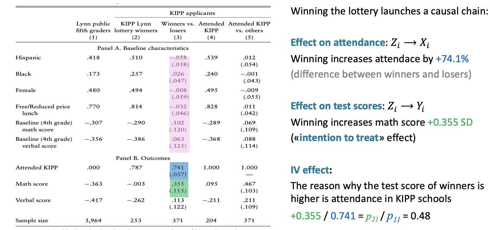
Not all students who win the lottery attend KIPP schools (only 74%). These individuals whose treatment status is determined by the instrument (the lotter) are called "compliers":

offer $= 0 ⟹$ KIPP $= 0$
offer $= 1 ⟹$ KIPP $= 1$

There are individuals that do not care about the lottery outcomes:

Always takers: attend KIPP wheter they win the lottery or not (4.6%)
Never-takers: never attend KIPP irrespective of the lottery (21.3%)
Defiers: who attent KIPP only if they lose the lottery (0%).

The IV estimate measures the Local Average Treatment Effect (LATE), which is the average causal effect of the treatment (attending KIPP) for the compliers.

the IV estimate does not provide information about the treatment effect for the always takers, never takers, defiers $⟹$ this because the IV method relies on the variation in the treatment caused by the instrument (and the treatment status of always takers, never takers and defiers is not influenced by the instrument)

Then the external validity of the IV estimate is limited because:

the IV estimate is limited to the compliers
the causal effect for compliers may not be the same of the causal effect for the entire population.

In the case of the KIPP study:

the IV estimate measures the causal effect of students attending KIPP schools because they won the lottery
it doesn't measure the effect of attending KIPP for always takers, never taker or defiers

$⟹$ the results are only valid for a subgroup.

Principles of Econometrics

Index

Note that the multiplicative error is <1 so the estimate is biased toward zero (attenuatoin bias).

Note that the multiplicative error is $< 1$ so the estimate is biased toward zero (attenuatoin bias).