Index
- Introduction
- Options and financial strategies
- Option valuation
- Pricing by arbitrage
- An introduction to the economic analysis of asset markets
- Choice under uncertainty
- Demand for risk
- Risk sharing and insurance
- Mean variance analysis
- CAPM
- Risk sharing and asset prices in a market equilibrium (CCAPM)
Suggested readings:
- Investments, Z. Bodie, A. Kane and A. Marcus, Fifth Edition, Parts IV and VI, for lectures 1 and 2 (later editions are available).
- Finance and the Economics of Uncertainty by G. Demange and G. Laroque, for the rest of the course.
0.1 Introduction - The Fama-Shiller controversy
In 2013, Eugene Fama, Bob Shiller and Lars Hansen jointly received the Nobel Prize in economics for their economic analysis of asset prices but, ironically, Fama and Shiller represent an interesting and controversial case for the subject.
Eugene Fama is most often considered as the father of the Efficient Market Hypothesis (EMH) which supports the Capital Asset Pricing Model (CAPM), which states that a stock's returns over time should be commensurate with its riskiness in relation to the overall market.
In formulas:
Where is the risk-free rate, (Beta) the sensitivity of the asset to the market, and the risk-premium (the extra return investors demand for picking risky assets over the risk-free).
Moreover, Fama argued that any test of EMH is actually testing two things at once:
- That the market is efficient.
- That the model is a correct way to measure risk.
Bob Shiller, on the other hand, published in 1981 the paper Do stock prices move too much to be justified by subsequent changes in dividends? that, answering Yes! to the question, claims that the EMH was one of the remarkable errors in the history of economics.
Regarding Fama's theories, Shiller's opinion was something like...
- I think that maybe he has a cognitive dissonance
- It's like being a Catholic priest and then discovering that God doesn't exist [...], you can't deal with that, you've got to somehow rationalise it.
In particular, Shiller’s empirical result is that stock prices move way more than the dividends.
If a stock price is truly the "discounted value of all future dividends", it should be stable because dividends don't change that much, but Shiller showed the opposite using the Cyclically Adjusted Price-to-Earnings (CAPE) ratio.
In the following years, empirical data gave credit to Shiller's critic.
But what does the CAPM actually say?
- how the market should price financial assets in function of the risk
- it shows that a complete market (perfect information and full pricing) will lead to a market equilibrium with optimal risk allocation
However, the CAPM relies on very heavy and simplifying assumptions, some are technical and could be relaxed, others are foundamental and not often realistic:
- the complete market assumption:
- it would require infinitely many assets
- it would require complex products (derivatives)
- complexity implies expertise and potential moral hazard
- other assumptions are unrealistic:
- investors can lend and borrow unlimited money under risk free rates
- all assets are divisible and liquid
- all agents have identical beliefs
So, was Fama simply wrong?
- Not really, he didn't give up and he refined the model, abandoning CAPM and replacing it with a multi-factor risk model
- Even Shiller still endorses a loose version of it.
- For Shiller, asset prices can overshoot in the short term (due to emotion and irrationality), but they show reversion to the mean in the long period.
- Additionally, according to Shiller markets are still the best tools we have for aggregating information.
To sum up, the Fama-Shiller case is typical from a social science and economics: two theories can contradict each other and still retain intellectual value.
"All Models are wrong, but some are useful" applies perfectly here: Fama gave an excellent structure to think the financial markets and, even if his work is imperfect, it's yet a solid starting point.
0.2 Introduction to finance and investment planning
A financial system is a set of institutions and markets that have the primary purpose of allowing the desynchronization of income and consumption.
A financial system allows to match different financial needs of different agents in two dimensions:
- Time (borrow and save):
- wish of continuous consumption vs discrete income stream
- smooth consumption of time/the life-cycle
- Risk (diversify, insure, hedge):
- smooth consumption across state of nature and possible market scenarios.
Asset: something valuable with well-defined property rights (a contract, a good).
Real Asset: something that has an intrinsic value due to its substance and properties.
Financial Asset: something that has NO intrinsic material value but which can be traded.
(Note that the distinction between financial and non-financial asset is not binary and well defined: for example, "is gold a financial or physical/real asset?")
Financial assets can be categorized as follows:
- Riskless assets: assets whose future values can be known with certainty (a government bond that yields 100 CHF in 5 years, assuming no default)
- Risky assets: assets whose future value may depend on some events (insurance, stocks, options)
- Derivatives are risky assets whose future values depend on the price of other assets.
A bond is often considered a riskless asset (depending on the issuer).
A zero-coupon (ZC) bond with maturity yields no payment before period and pays in period .
They can vary only in terms of maturity.
Denote by the price of a ZC bond with maturity at time (usually the first subscript is current time, the second the maturity). In absence of arbitrage, we have:
where is the discrete per period forward interest rate between and . By iteration we have:
In relation to this, we can distinguish:
- Discounting: the process of determining the prevent value of a future payment at time :
- Compounding: the process of determining the current value at time (in the future) of a monetary amount invested at
The discrete spot interest rate , for a zero coupon bond with maturity such that:
Or, in other words, the spot rate is the geometric average of the per period forward rate of interest:
We now consider a bond with price in that yields a series of positive coupon payments until the maturity date, so for , plus the final payment of par value in .
Its yield to maturity(YTM) is the unique rate for which the present value of these payments is equal to :
The same analysis can be formulated in continuous time, in this case the instantaneous forward interest rate is:
or, equivalently:
By integration, we get:
This interest rate is called "instantaneous" since it represents the evolution of the bond's price process for an infinitesimally small period of time .
Moreover, in continuous time we can define:
The continuously compounded forward interest rate between , denoted by is defined as:
The continuously compounded spot interest rate for a bond with maturity is:
which is the arithmetic average of the instantaneous forward interest rates between .
The function provides the yield curve.
We now consider risky assets. To evalute an uncertain stream of future payments, we still used an additive process:
where the second formulation is needed if we want risk to be taken into account, and we write , where is the risk-free rate and the risk premium.
1. Options and financial strategies
Derivatives are assets whose values mechanically depend on the values of other financial assets (the underlying).
For example:
- Forward contracts: OBLIGATION to purchase (long position) or sell (short position) the underlying at a specified future price at a specified delivery date.
- Options contracts: RIGHT to purchase or sell a specified amount of the underlying at a specified exercise price at or before a specified expiration date.
Options offer an advantage: the transaction does not have to occur if it is not profitable for the owner of the option. This advantage comes at a price:
- Forwards are entered at NO cost
- Options are purchased or sold at positive price that represents the cost of the right to buy/sell.
- Selling (or writing) an option implies an obligation (if the option is exercised, the seller must sell or buy the stock and incurs a loss) the seller receives a compensation.
Derivatives can help shaping the risk exposure:
- Hedging means insuring against market price volatility
- Speculation means expoiting market price volatility
Forward Contract Payoff
- agreed delivery price
- spot market price of the underlying at maturity
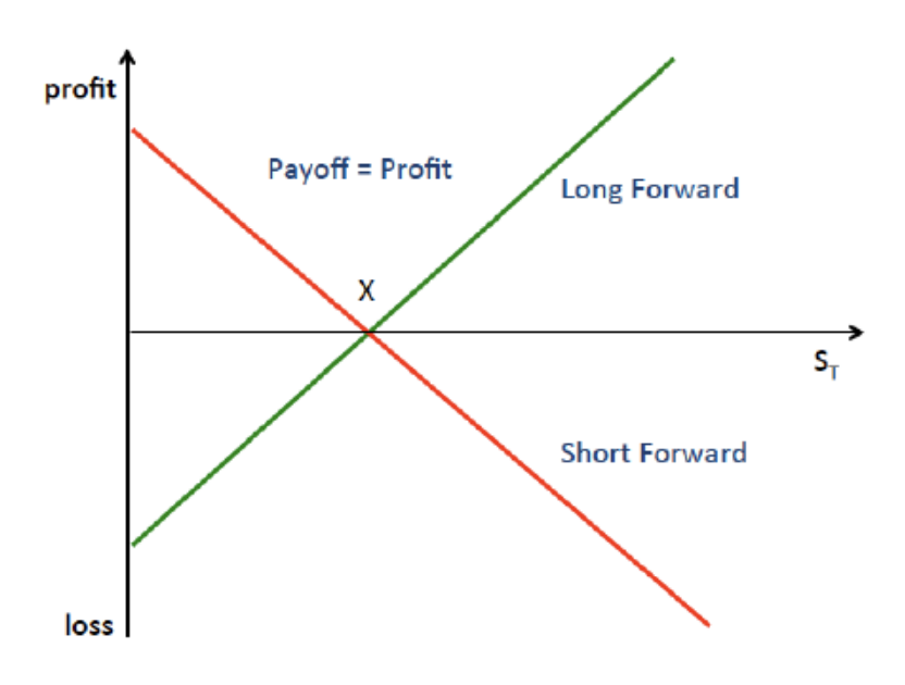
Profits at maturity are:
- Payoff long position
- Payoff short position
For this reason, forwards are great for speculation. At a given time , an underlying has a price , with no clear evolution for the future. If a speculator expects:
- long forward with
- short forward with
On the other hand, forwards are used in hedging to avoid risks.
Suppose, for example, that Giacomo's GmbH needs to sell an activity (example: some running shoes) at maturity , with value at given time .
Giacomo faces then a risk management problem: how can he insure against price fluctuations of the running shoes?
Solution: use the forward contract to construct a hedged portfolio that fixes the profits from the future sale at a desired level :
To fix the profits at , Giacomo can open a short position on the forward contract with delivery price .
(The opposite - long forward contract - applies if you need to buy and you want to avoid risk).
Options Payoff
An option is a right to purchase/sell a certain amount of the underlying at/before future expiration at exercise price (strike) .
Options differ by:
- Position
- Long: option holder (right to exercise)
- Short: option writer (obligation to facilitate the option's exercise)
- Type of right:
- Put: long position has the right to sell an asset for
- Call: long position has the right to purchase an asset for
- Possibility of early exercise:
- American option: exercise at or before expiration
- European option: exercise only at expiration.
Consider now:
- exercise price of an option
- market price of the underlying at expiration
- Premium: purchase price of an option (market value):
- : premium for a call at
- : premium for a put at .
Payoff/value at expiration:
| Condition | Call: Long Position | Call: Short Position | Put: Long Position | Put: Short Position |
|---|---|---|---|---|
| 0 | 0 | |||
| 0 | 0 |
Profits are then given by:
- Long position:
- Short position:
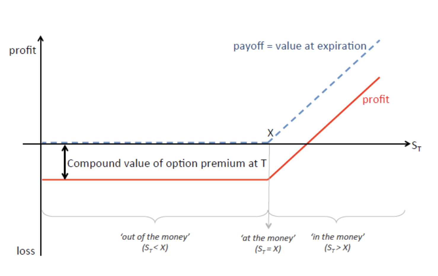
Long Call
Short Call
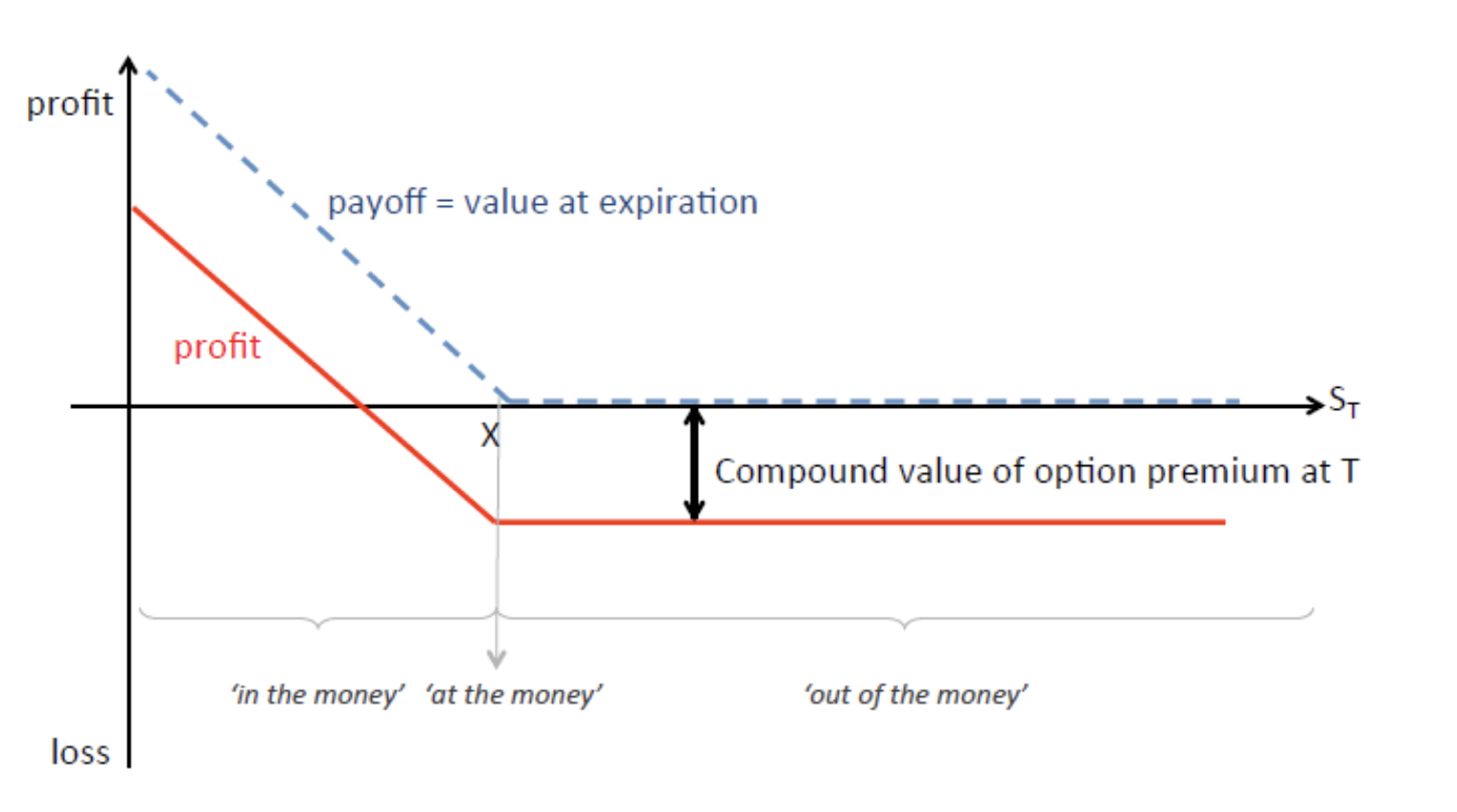
Long Put
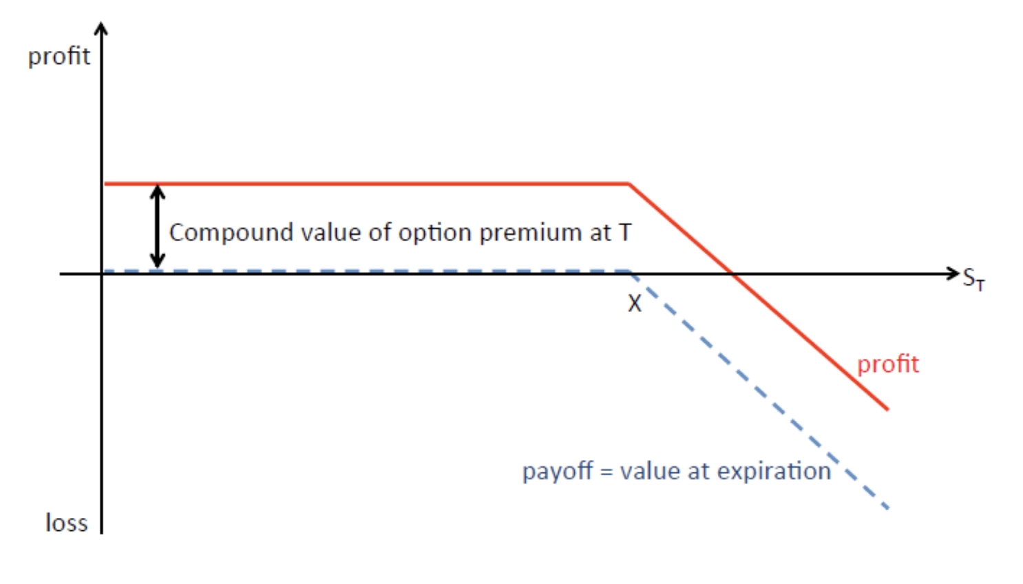
Short Put
Option Strategies
If the agent has an expectation about the price development of the underlying:
- Bullish strategies: generate a profit when the underlying's price increases
- Bearish strategies: generate a profit when the underlying's price decreases
- Non-directional strategies: generate a profit depending on the underlying's actual volatility.
But... what are the reasons for trading in options rather than trading in the underlying directly?
- Leverage effect: option values respond more than proportionately to changes in the underlying's value.
- Tailoring risk exposure of investment: options can be less risky due to limitation of the downside risk.
- Portfolio insurance: it can be insured by long on a put for that stock.
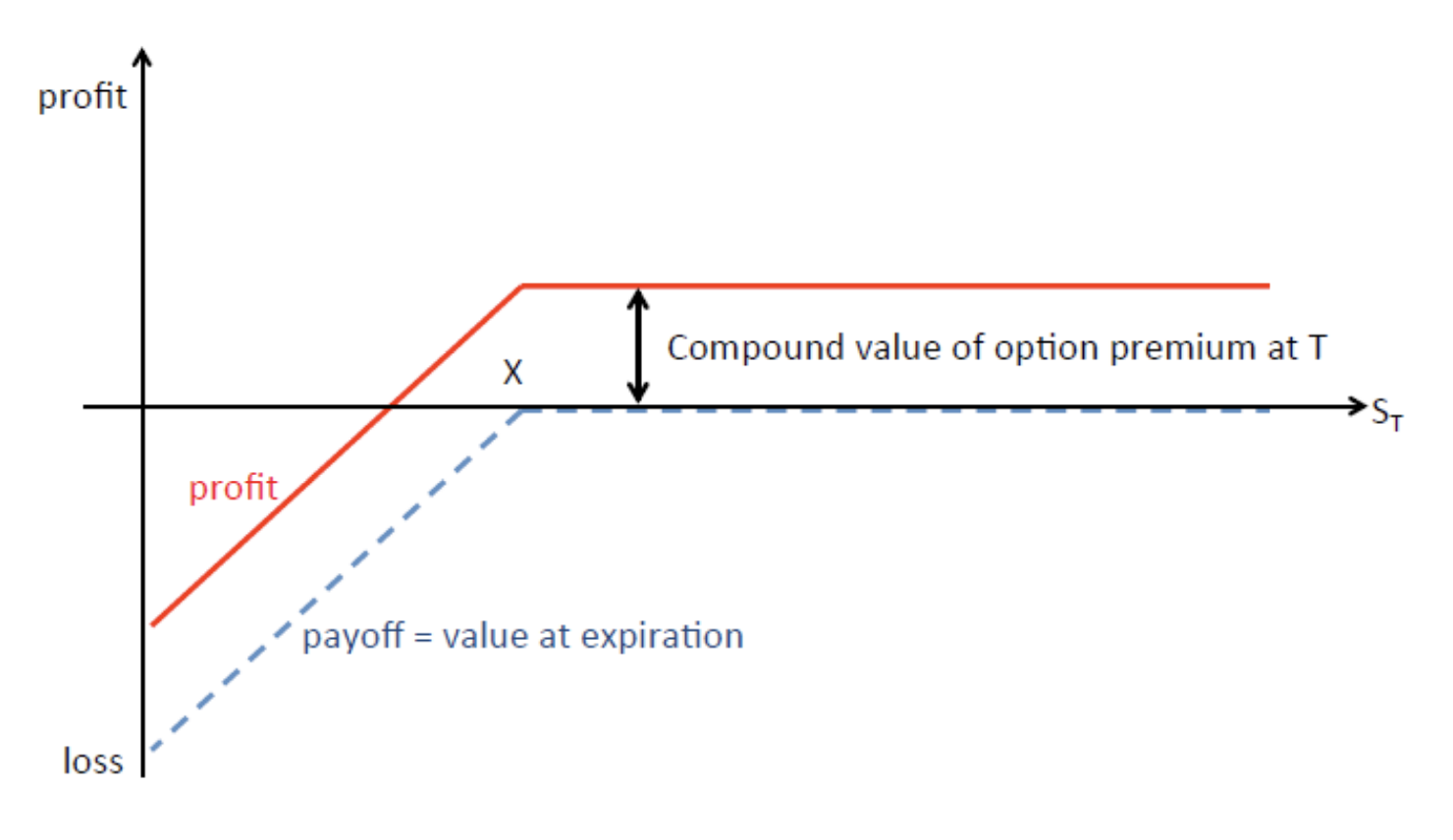
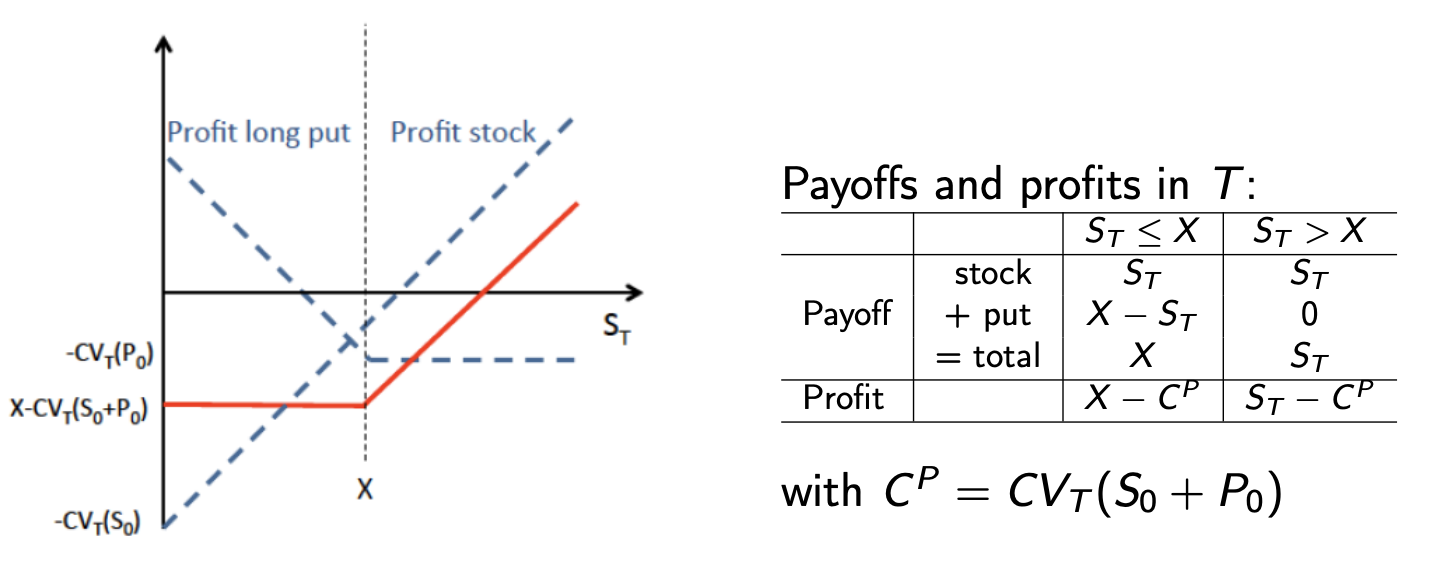
Option strategies: Protective Put
Consider an agent that:
- invest in a stock with price
- wants to insure against potential declines in the stock price
long put on the stock (exercise price in with premium )
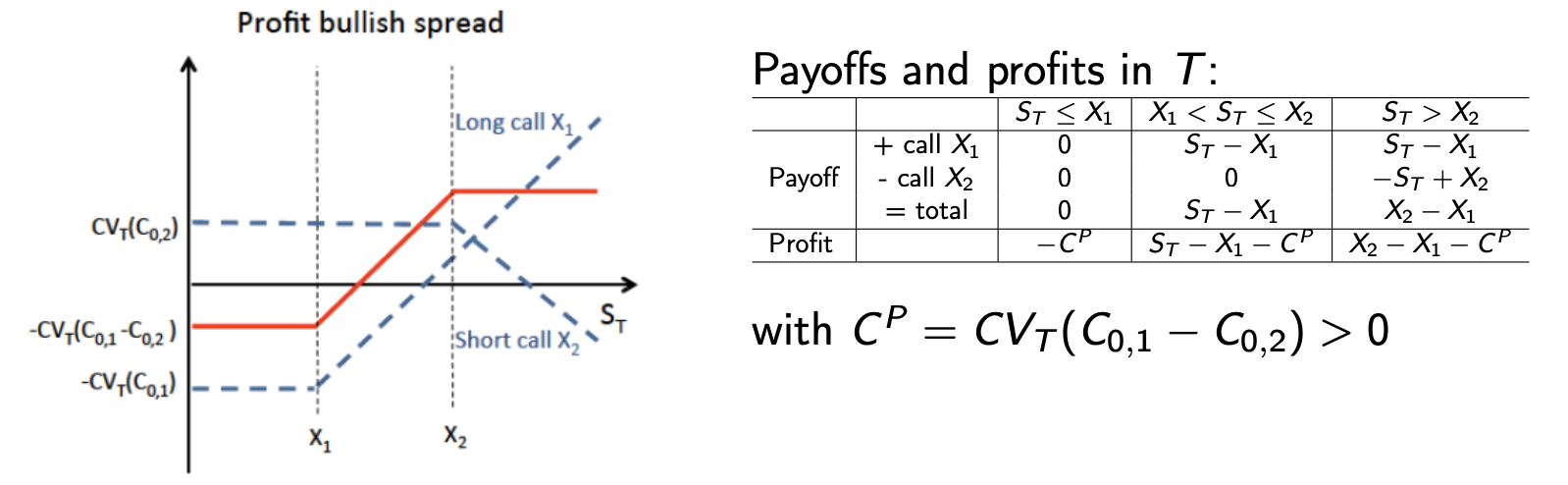
Option strategies: spreads (I)
Consider an agent that wants to take advantage of higher future price of the underlying.
He could buy the stock, buy a call or short a put, or as an alternative, construct a portfolio that allows to reduce the risk at the cost of _giving up part of the profits:
This is called Bull spread strategy:
- 1 long call with strike and premium
- 1 short call with strike and premium
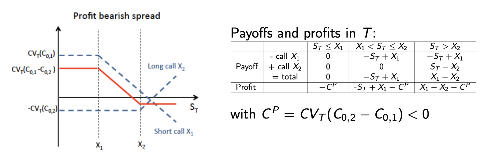
Option strategies: Spreads (II)
The opposite also applies, i.e. consider an agent that wants to take advantage of lower future price of the underlying.
Bear spread strategy- 1 short call with strike and premium
- 1 long call with strike and premium
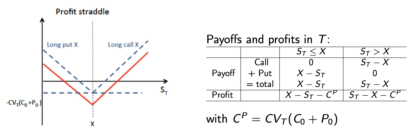
Option strategies: Straddle
Consider an agent that expect large move in the stock's price but he's uncertain about the direction.
Straddle Strategy:
- 1 long call with strike and premium
- 1 long put with strike and premium
Moreover, if he thinks:
- a stronger bullish move is expected: buy 2 calls and 1 put (long strap)
- a stronger bearish move is expected: buy 2 puts and 1 call (long strip)
2. Option valuation
In this chapter we focus on European options, please refer to the above sections for formal definition.
We also use the following notation:
- : price of the underlying asset at toime
- : prices (premia) of the call and the put option at time .
- : rate of the risk-free asset.
An Arbitrage Opportunity is defined as a financial strategy that yields a (sure) cash flow at time and a cash-flow at time and there is at least one stat of the word where one inequality is strict.
- almost surely is an arbitrage
- almost surely with is an arbitrage
In this chapter, we assume that the market is arbitrage-free (the market clears out arbitrage opportunities).
Price Bounds on call options (European, no dividend)
- Upper Bound:
Proof:
Consider two portfolios:
-
Portfolio : call + cash $PV(X)
- Price in : $ [C_0 + PV(X)]
- Value in : $X + \max [S_t. X, 0] = \max [S_t, X]
-
Portfolio : stock
- Price in
- Value in :
Portfolio is never less valuable than portfolio in , so cannot be less expensive in , otherwise we have an arbitrage opportunity, therefore we conclude:
and since the call is an option.
- Lower Bound: where is the present value operator.
Price Bounds on put options (European, no dividend)
- Upper bound:
- Lower Bound:
Proof:
Consider two portfolios:
- Portfoio : buy put + stock
- Price in :
- Value in : ]
- Portfolio : cash
- Price in :
- Value in :
is never less valuable than , so cannot be less expensive in , otherwise we have an arbitrage opportunity, therefore:
and we add since the put is an option.
The Put-Call Parity Theorem
To understand this, consider the following:
- Portfolio : stock and put
- Portfolio : bonds and call
the values of the two portfolio are equal in , therefore they have to be equal also in , leading to the Put-Call parity formula.
Option Valuation
Determinants of the value (price/premium) of a call option (European, no dividend):
- stock price (+), exercise price (-)
- volatility of underlying stock (+) (intuition: volatility increases the probability that the stock value at expiration is greater than , increasing potential gains).
- time to expiration (+) (intuition: the more time to expiration, the higher the range od stock price increases, similar to volatility), also, the present value of exercise price falls)
- interest rate (+) (intuition: present value of exercise price falls).
Two-state Option Valuation Model
Consider a market with:
- a stock that currently trades at , and which value in can be either , with
- call option on the stock with exercise price and expiration date
- a risk free asset with yearly interest rate
Then it is possible to replicate the payoffs of the call using a combination of the risk-free asset and the stock. The replicating strategy can be found as:
which gives:
In absence of arbitrage, since the price of the replicating strategy and the option must be the same , we can conclude that:
Intuition: in case of arbitrage, given the put-call parity formula we can construct an arbitrage opportunity by shorting the "cheapest" side and going long on the "expensive" one.
Note that the same reasoning (with different derivations) can be applied to any payoff.
We can now apply the same reasoning in continuous-time.
Considering a given time range , we split the time range in (infinitely many) periods and we assume that in any period the stock price is multiplied by either .
We assume the distribution of the stock price at time is log-normal.
Applying (infinitely many times) the two state valuation model makes it possible to compute the value of the call.
Black-Scholes Formula
Formally, the value of the stock at time denoted is assume to vary as follows:
where is a standard Brownian Motion, so for any the distribution of is log-normal.
We then assume:
- constant risk-free interest rate
- no arbitrage
and we get the famous Black-Scholes formula:
-
-
-
probability that a random draw from a standard normal distribution will be less than
-
: risk free interest rate, (annualized continuously compounded rate with same maturity as the expiration of the option, note that is different from ),
-
: standard deviation of the annualized continuously compounded rate of return of the stock.
Intuition: can be interpreted as the risk-adjusted probabilities that the call option will expire in-the-money ()
The Trillion Dollar Equation [VIDEO - Veritasium]3. Pricing by arbitrage
We consider two periods: ex-ante, ex-post, denoted by and contingent states at time .
There are assets available at time .
- is the value of asset in state at time
- we denote the price of asset at time
- a market is the data:
A portfolio is a vector of asset quantities: is the quantit of asset in the portfolio.
- the price of portolio is:
- the value of the portfolio in state is:
Given now a market with:
a portfolio with asset quantities has price:
and values
We then introduce the followig definitions:
- an asset is risk-free if is independent of
- an asset can be replicated by a subset of assets, indexed , if there exists a constant such that:
(in such cas the asset is called redudant).
A market is complete if for any asset there exists a constant such that:
In other words, the market is complete if the payoff matri has max rank:
where is the number of states.
On the other hand, markets are complete when all revenue configurations are replicable through some portfolio.
Consequences of complete markets:
- there are at least as many assets at the states:
- a market is complete if and only if the payoff matrix ith dimension has rank .
- if a market is complete with , there are independent assets, then we can eliminate assets which are linear combinations of the independent ones.
An arbitrage portfolio is a portfolio such that:
at least one of these inequalities being strict.
A market is arbitrage free if there is no arbitrage portfolio.
Law of One Price
A market without arbitrage opportunity satisfies the Law of One Price:
If two assets satisfy for every state , then the two assets have the same price .
More on the law of one price [Investopedia].
ProofAssume that , then the portfolio such that for satisfies the following:
that is an arbitrage portfolio.
The No-Arbitrage Theorem
A market is arbitrage-free is and only if there exists a vector such that:
- for every state
- for every assets
is then called state-price vector.
In matrix form, the state-price vector with positive components solves:
There may exists several state price vectors in a market.
Intuition:
- the state price () is simply the price you must pay today to receive that in state tomorrow (regardless of the asset).
- the state-price vector is just the collection of these prices for every possible future state.
- doesnt tell you which assets to buy to receive
- once you have the state-price vector , you can price any asset using the sum above (the price of an asset equals the sum of its payoff in each state weighted by the state prices)
Risk Neutral Probability
Assume a state price vector .
Denote , with .
Therefore can be interpreted as a probability. In particular, is called the risk neutral probability.
- if a market admits several state price vectors, it admits also as many risk neutral probabilities.
If we define: the return of asset in state , using :
If we substitute the definition of :
If we extract the constants ( and the total sum of state prices) out of the summation:
Since is exactly the definition of , the terms cancel out:
All asset returns have the same-risk neutral expectation. (This does not imply that all assets have the same returns expectations according to physical probability).
For any state , the corresponding Arrow-Debreu security, denoted by , is the asset with values given, for all , by:
- If the market is arbitrage free and is a state-price vector, then the price of is .
- A market that contains all Arrow-Debreu securities is complete.
Intuition: a contract that pays exactly if a specific state of the world and in every other possible scenario.
Assume now that a market includes a risk-free asset that pays in all state of the world and denote by its price () and , then:
- for all assets :
- if the market contains the Arrow-Debreu security , its price is
Arbitrage Bounds
Given an arbitrage-free market , define the set of state price vectors for this market:
- is a convex set
- empty offers arbitrage opportunities
- is reduced to a point M is complete and arbitrage-free
- if , then , that means:
Theorem (Arbitrage Bounds)
For amy claim , not necessarily replicable in , the set of prices for such a claim to not generage arbitrage opportunities is:
- this set is singleton is replicable in
- if is not replicable, the adding it to the market with a price within arbitrage bounds will reduce (dimension decreases by one)
4. An introduction to the economic analysis of asset markets
Some introductionary definitions for the following chapters:
| Ex-ante | Ex-post | |
|---|---|---|
| Knowledge | → Possible states of the world occurring with known probabilities | → Realization of state; → Income received |
| Action | → Contract/commit on what will happen ex-post | → Implement the contracts; → Consumption |
| Action in a market setting | → Purchase/sell assets | → Realization of assets' payoffs; → Consumption |
We begin this chapter with a simple example about market equilibrium.
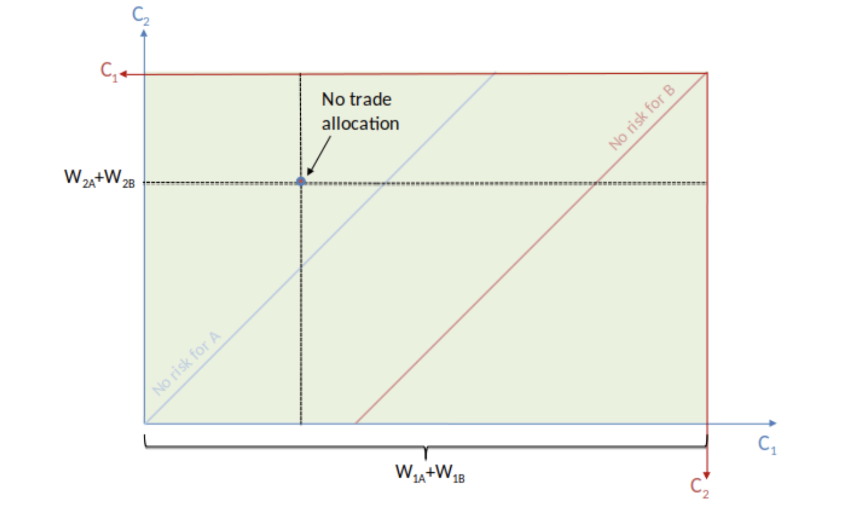
Consider two agents and two-states of the world (ex-post) :
- in state , agents get income
- in state , agents get income
Denote then by their consumption.
The feasible allocations must satisfy:
The no-trade situation corresponds to and .
In this chapter, we rely on the standard specification for the Expected Utility Theory:
where are the probability for scenario and is the utility index function.
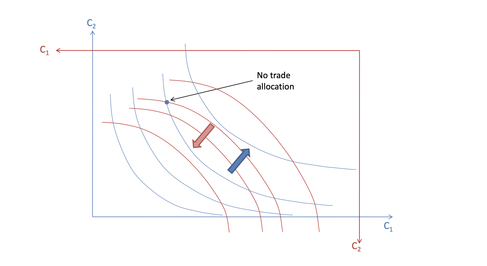
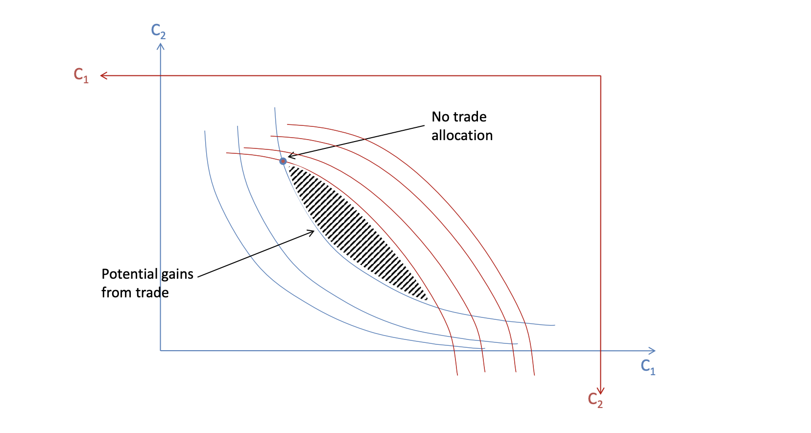
An allocation is Pareto-optimal there is no alternative feasible allocation at which every individual in the economy is at least as well off and some individuals is strictly better off.
Graphically, Pareto-optimal allocations are the ones where the indifference curves are tangent.
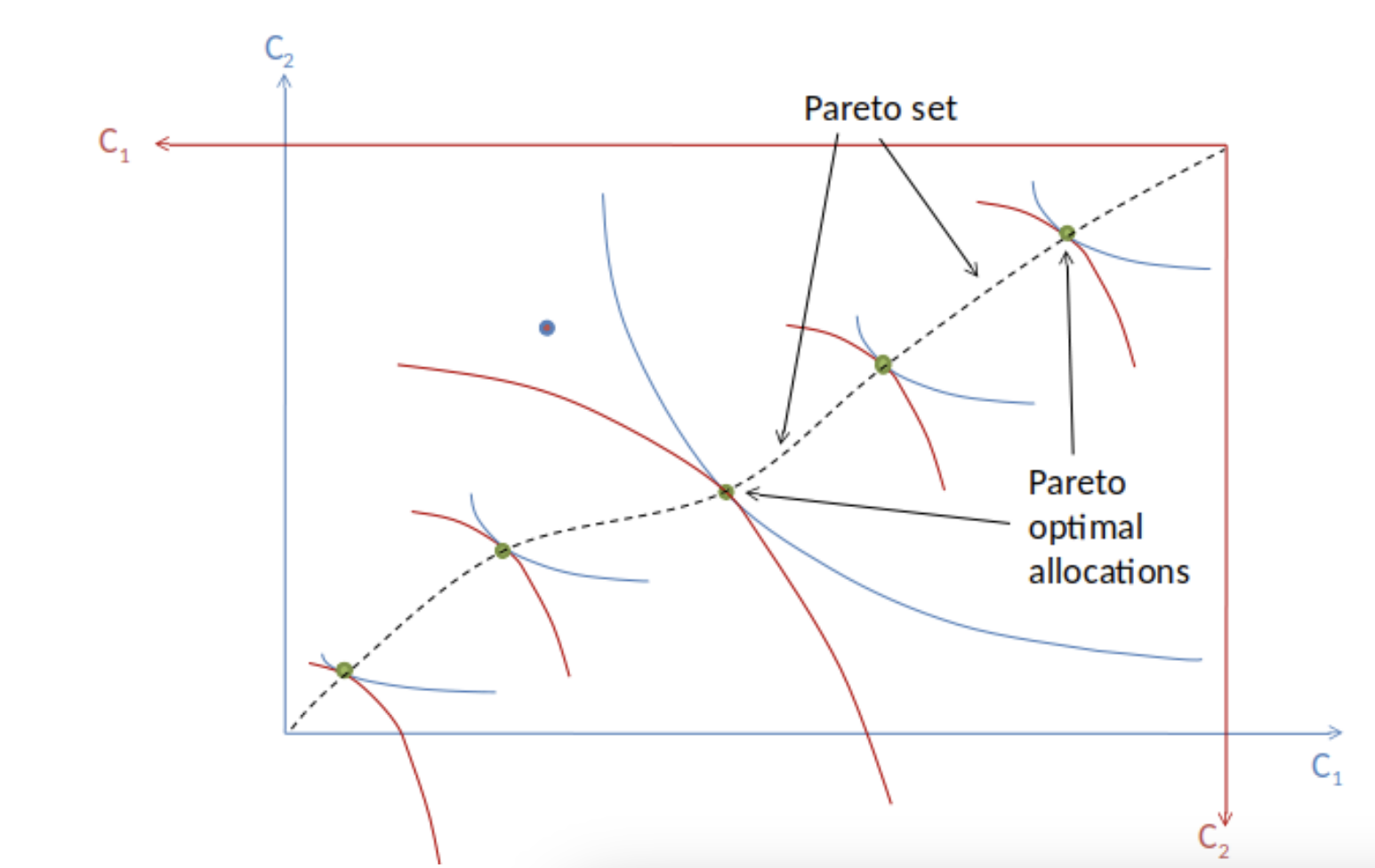
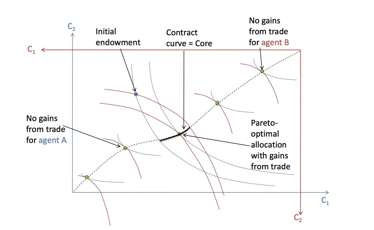
The contract curve (or core) is the part of the Pareto set for which both agents do at least as well as their initial endownets. On the core, both agents gain from trade and the outcome is Pareto-optimal.
Agents interact by trading assets on a market:
- assets are purchased/sold ex-ange (before uncertainty realizes)
- payoffs are given ex-post
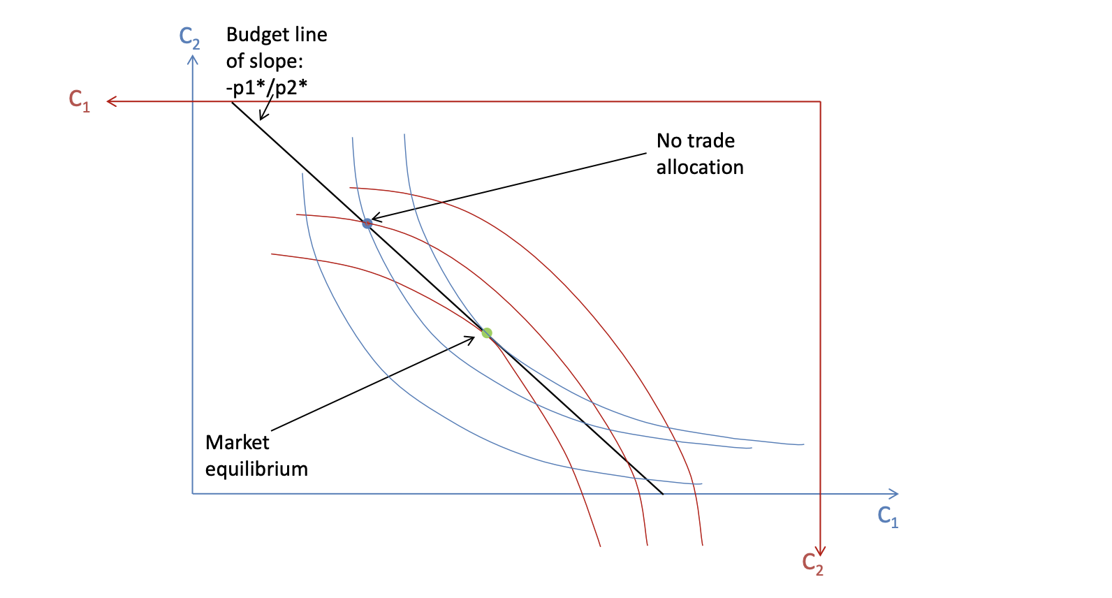
- market equilibrium occurs when asset prices are such that individual strategies are globally compatible (demand = supply).
A Complete Market
We consider two assets (Arrow-Debreu Securities) in a two-states world:
- A risky asset :
- it can be purchased/sold ex-ante at
- ex-post it pays for and zero otherwise
- A risky asset :
- it can purchased/sold ex-ante at
- ex-post it pays for and zero otherwise.
denote the quantities of assets for agents (they can be positive or negative depending on purchase/sell).
Ex-ante, each agent has zero initial wealth and a budget constraint:
Ex-post, assets' pay-offs and income and realize and agent consumes .
Therefore, agent solves the following optimization problem:
This problem generates the demand functions:
Market ClearingA market is balanced (cleared) when demand equals supply for all assets (Market Clearing Conditions):
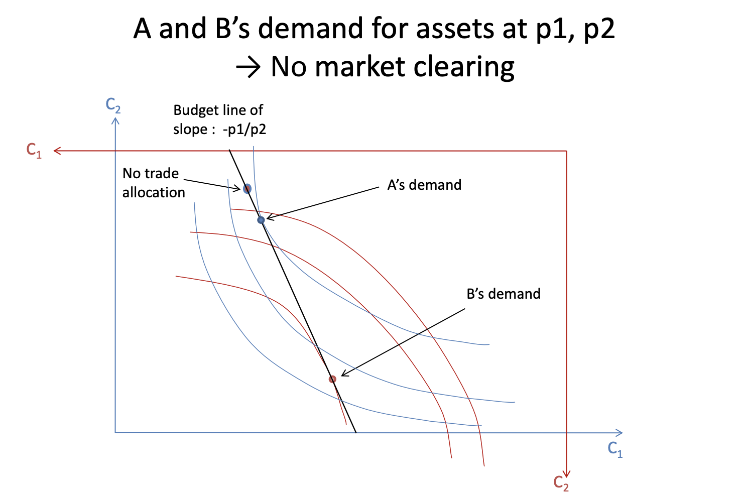
At equilibrium, we then have 2 equations in 2 unkwnowns:
Considering also the budget constraints, the previous two equations are then equal, so we have independent equation and unknowns.
Equilibrium prices are determined up to a multiplicative scalar.
The following plot shows risk transfer: A has NO income risk, but rather takes some risk from B.
The allocaitons are comonotonic if and only if:
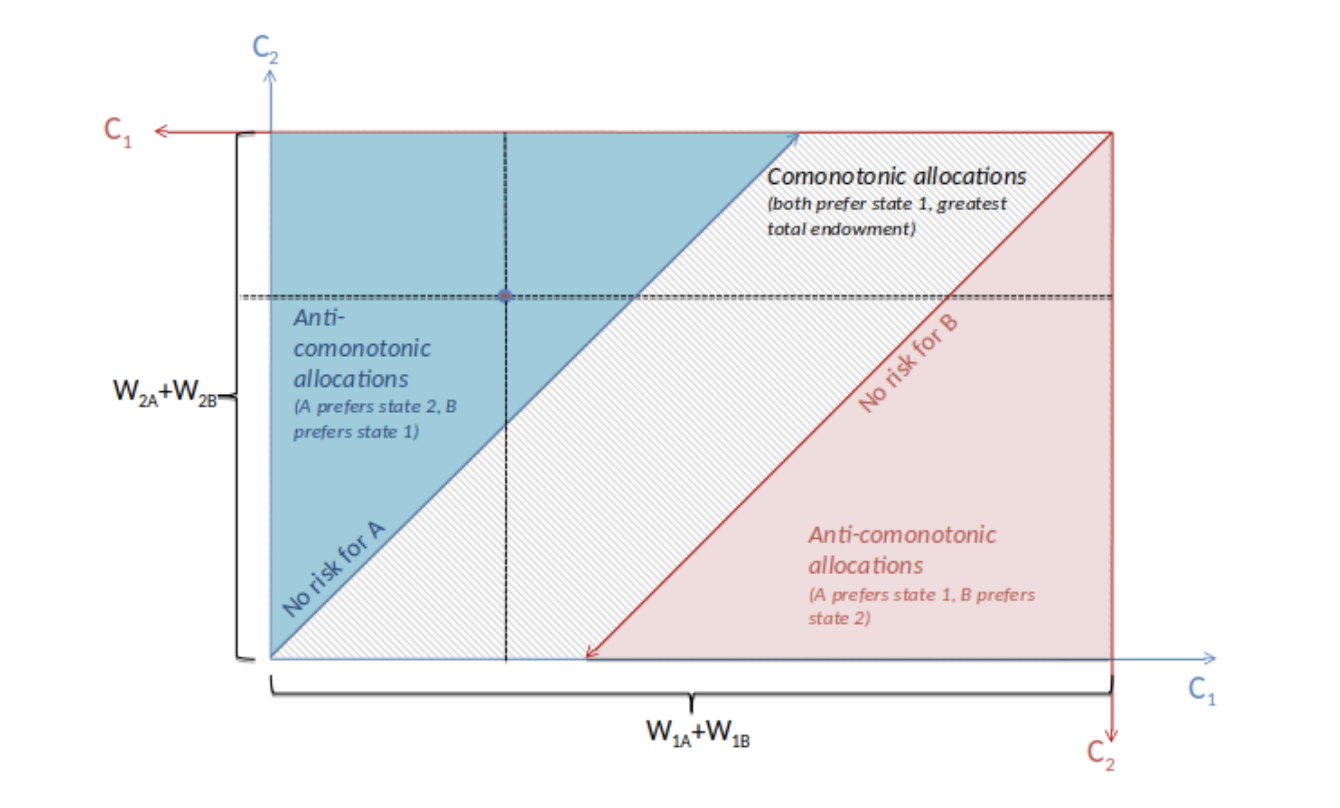
All market equilibrium allocations are comonotone, this is also the case for Pareto-optimal allocations.
Price responseto changes in risk
Consider now the case where 's endowment in state decreases, so is smaller.
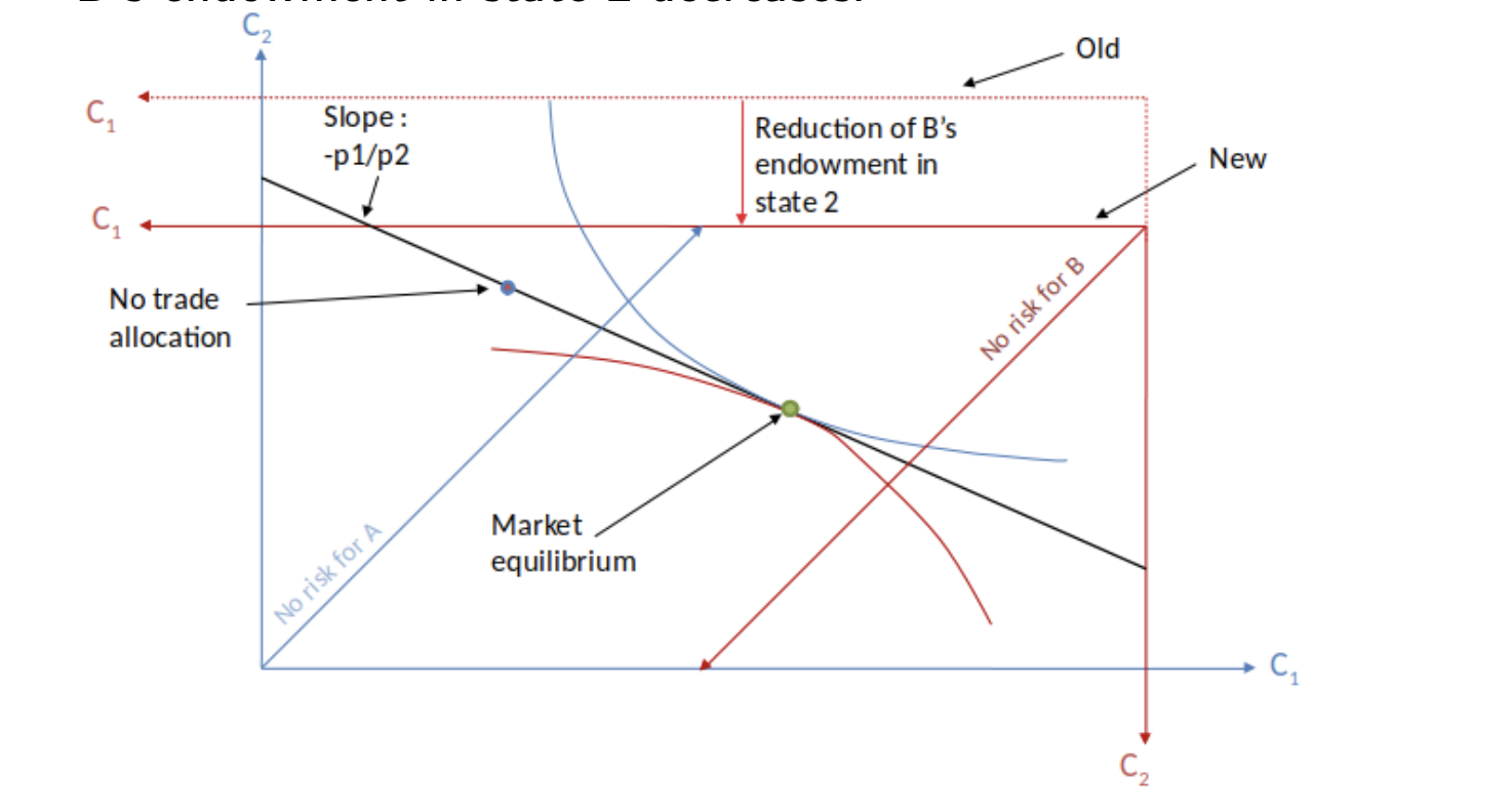
In this case, an increase in the risk of leads to take more risk.
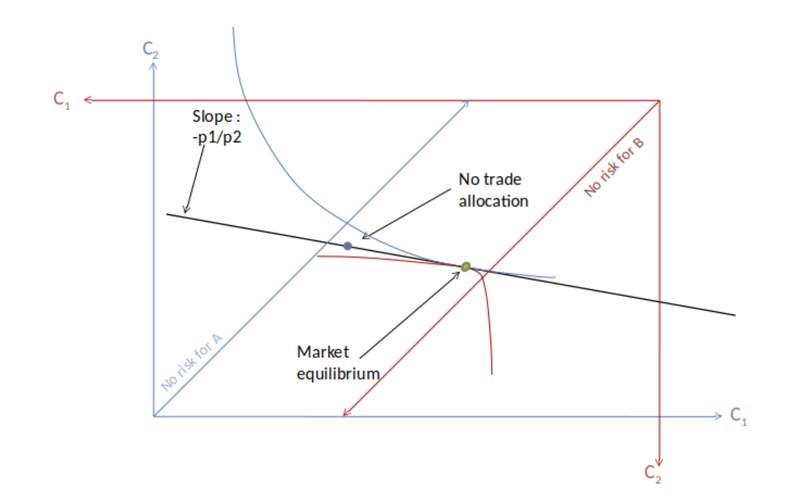
In general, low risk averse agents take the most of the risk.
An interactive simulation of risk preferences can be found here.
5. Choice under uncertainty
Consider a set of possible consequences. Let the set of possible states of the world and the set of lotteries with consequences in .
A lottery is a list of pairs where gives the probability that will occur, and is the outcome.
Example: is the lottery that pays with equal probabilities.
A compound lottery is a lottery whose prizes are themselves lotteries.
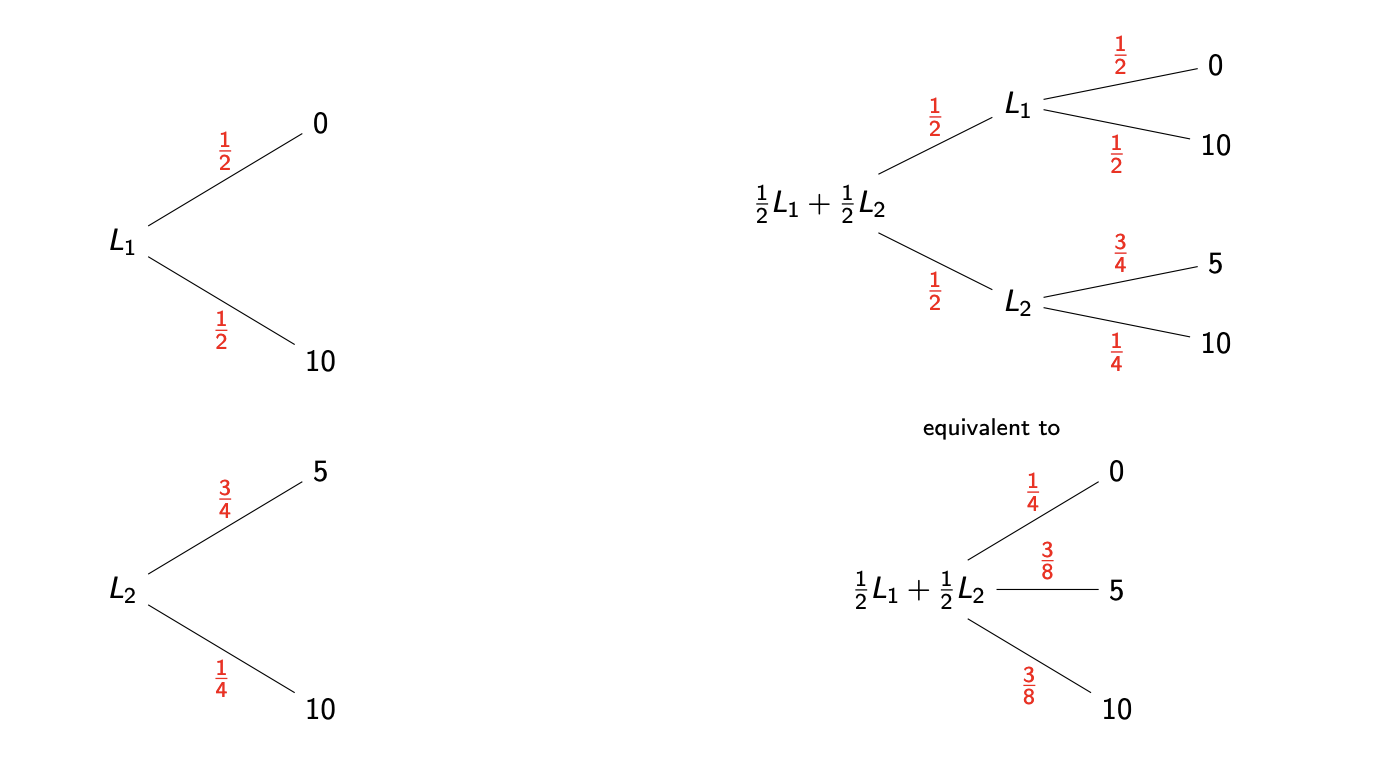
Mixture operationConsider two lotteries .
The compound lottery with corresponds to the lottery which consists in playing the first lottery with probability and the second with probability .
The resulting lottery is denoted by . The operation + is called a mixture operation.
Example:
Preference Relation
We want to define a theory of preference defined over .
A relation of preferences on is a binary relation which is:
1.Complete
- for any , we have or
-
Transitive
- and
Axioms of Expected Utility Theory
Von Neumann and Morgenstern suggested to assume the following about the relation of preference:
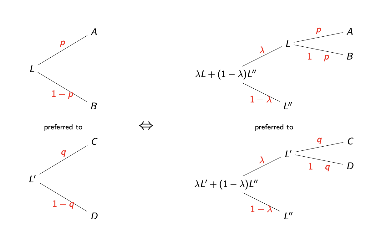
- Independence: for all and :
- Continuity: if , then there exists such that .
Graphically, the independence axiom:
A relation of preferences is represented by a utility function if and only if: .
Theorem (Von Neumann-Morgenstern)If is a preference relation on that satisfies the previous axioms, then there exists such that:
that can also be rewritten as:
In this case, we say that the agent is said to have "VNM preferences".
A little note on terminology:
- is the utility function (expected utility function).
- is just a function that appears when looking at the structure of (utility index). Furthermore, for the rest of the chapters, we assume that is strictly increasing and twice continuously differentiable.
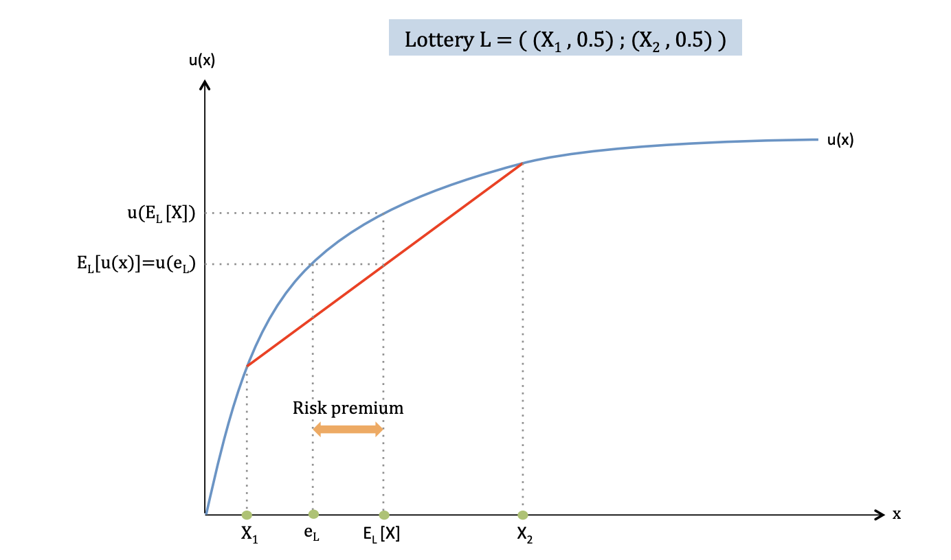
Risk Aversion
We denote the average of lottery by .
We represent with the degenerate lottery that gives the expected payoff of with probability one.
An agent is said to be risk averse if and only if for all :
An agent with VNM preferences is risk averse if and only if her utility index is concave: .
To prove it, we consider the Jensen Inequality: if a function is concave, then we have:
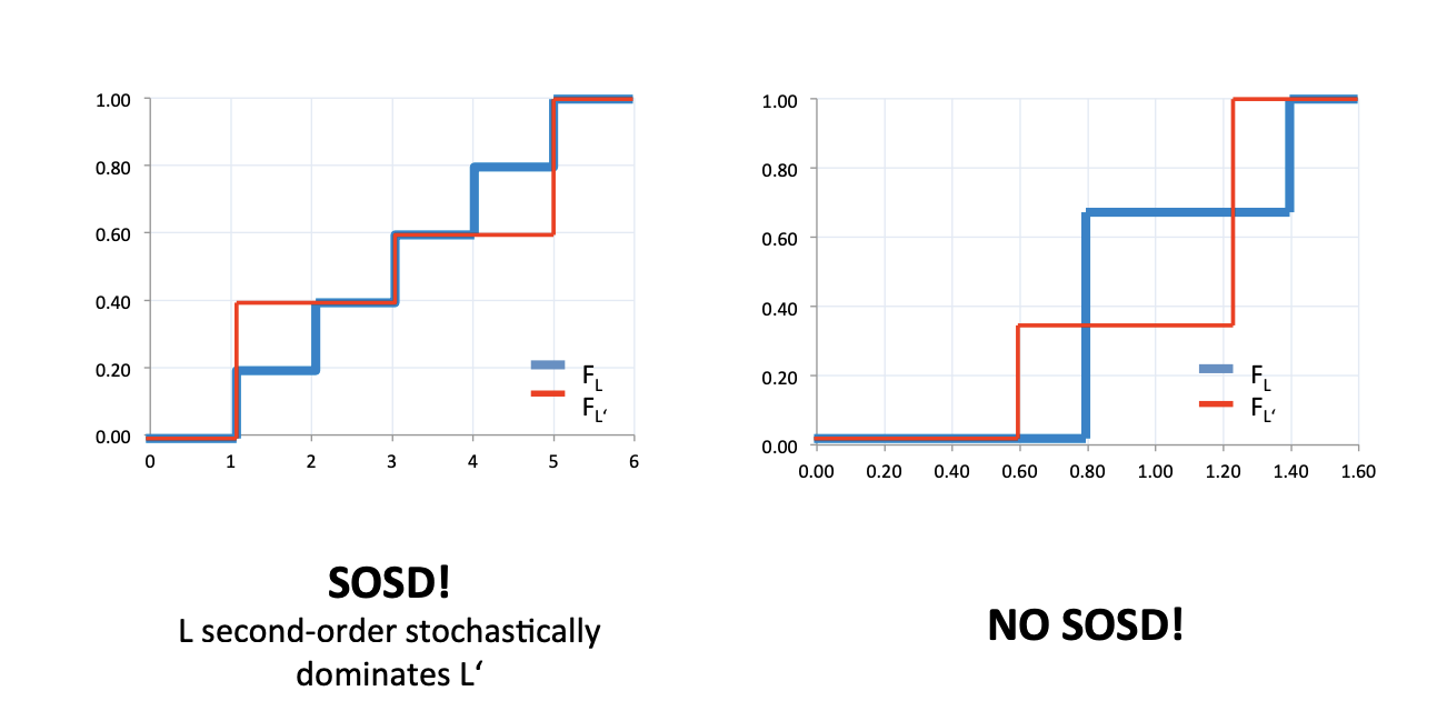
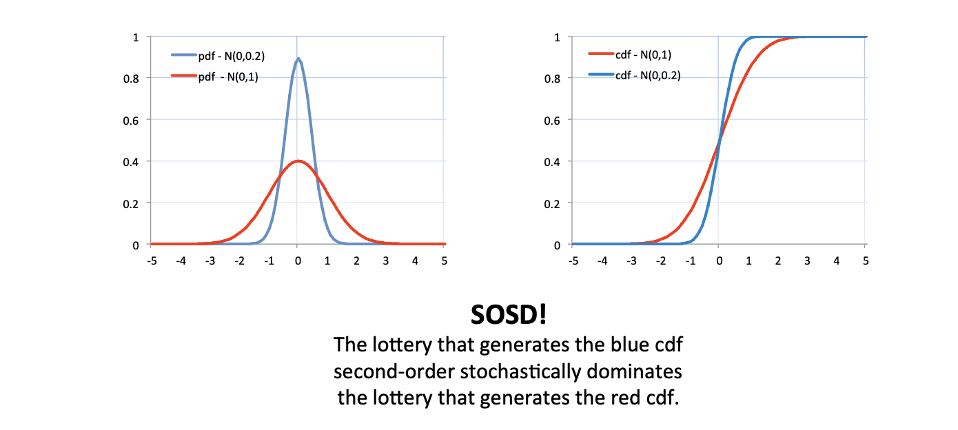
Recall: for any lottery we can define the cumulative distribution function as:
Second-order Stochastic DominanceA lottery is said to second-order stochastically dominates if and only if: and:
(Note that the first order stochastic dominance implies the second one)
Clearest Explanation of Second-Order Stochastic Dominance! [VIDEO]
Understanding First-Order Stochastic Dominance[VIDEO].
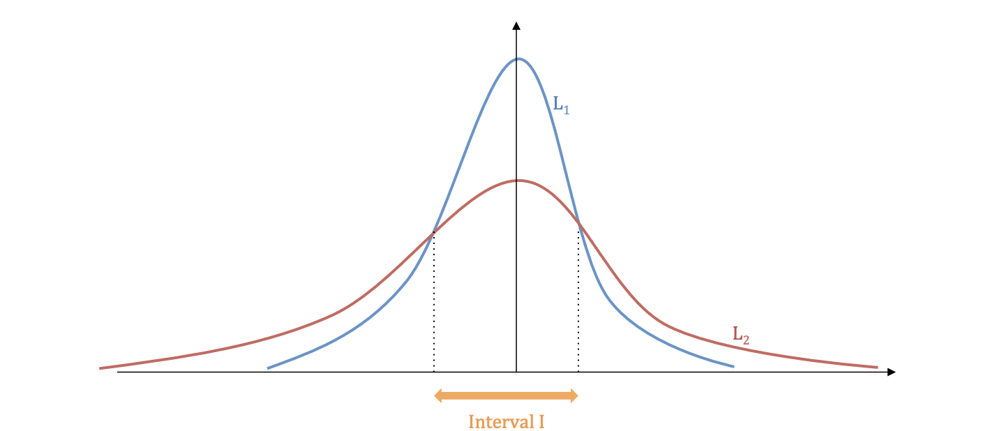
Mean Preserving Spreads
Consider with the same mean and with density functions . is said to be a mean preserving spread of if there exists an interval such tat:
Increases in Risk
There are different ways to define an increase in risk:
- is riskier than if ( second order stochastically dominates ).
- is riskier than if is a mean preserving spread of .
- Adding a white noise: is riskier than if , where . (Note that do not need to be independently distributed).
An agent with VNM preferences dislikes increases in risk if and only if her utility index is concave.
Quantifying Risk Aversion - Certainty Equivalent
For a lottery , its certainty equivalent is amount such that: or, in other terms:
Intuition: is the amount of money for which the individual is indifferent between playing and a fixed amount of money.
- For a concave utility (risk averse agent):
- For a linear utility (risk neutral agent):
Risk Premium
For any lottery with payoff , define the certainty equivalent as:
The risk premium is then:
For a VNM agent, this is equivalent to:
- A risk neutral individual has zero risk premium
- A (strictly) risk-averse agent associates a positive risk premium to any non-degenerate lottery.
Intuition (preference rule): a VNM agent (risk-averse) always prefers the lottery with the higher certainty equivalent. If the lotteries have the same mean , the agent prefers the one with the smaller risk premium.
Absolute Risk Premium for small risksConsider , small and the following lottery:
Using Taylor expansions, we can show that the (absolute) risk premium when is small (Arrow-Pratt approximation) is such:
The absolute risk aversion coefficient for wealth level is defined as:
For small risks of the form :
Note that is the variance of the risk.
Relative Risk premium for small risksConsider and the same lottery as before, .
We can define the relative risk premium by:
and, using the Taylor expansion when is small:
The relative risk aversion coefficient for wealth level is then defined as:
For a small risk of the form :
Comparing Risk Aversion
For two agents all the following sentences are equivalent:
- the certainty equivalent of is smaller or equal than the one of .
- the risk premium for is smaller or equal than the one for
- is more concave than : there exists and increasing concave functio such that: .
- we have:
- is at least as risk averse as
Common Classes of VNM utility indices
- Costant Absolute Return Aversion (CARA)
- Constant Relative Risk Aversion (CRRA)
- Hyperbolic Absolute Risk Aversion (HARA)
- Quadratic Utility Index
Note that for a quadratic utility index:
then the utility of a lottery only depends on its mean and variance.
6. Demand for risk
Static Portfolio Choice - Setting Up the ProblemConsider an agent with wealth who can invest at time zero in a risk-free asset with return and in a risky asset with random return .
If the agent invests in the risky assets, he gets in period :
with and , the agent's problem rewrites as:
Positive Demand for Risky AssetLet's start deriving some properties:
Then if the agent is risk-averse, is concave and therefore is non-increasing, so we can conclude that:
- if : the agent should purchase some risky asset (regardless of how much risk averse he migh be).
- if : it is never optimal to purchase the risky asset.
Static Portfolio Choice - First Order Conditions
We derive the first order conditions to quantify how much the agent should invest.
- If is always of the same sign there is no interior solution.
- Even if the agent is risk-averse and changes sign, there may not be an interior solution.
In the following, we assume that there exists an interior solution and that , so that the solution is positive ().
Static Portfolio Choice - Small RisksWe assume , with and .
We denote by the solution to:
from which we can derive the first-order condition:
We know that , so using a Taylor Approximation, we expand around .
Since (at zero mean excess return, the agent doesn't buy the risky asset), the first-order Taylor expansion is: .
We then substitute into the wealth argument, so the final wealth is:
Substituting :
We then expand around , using :
The term is second-order in , so we drop it:
Since , for small we can write this as:
If we plug it into the first-order condition, we obtain:
that finally gives:
Then the share of wealth invested in the risky asset is:
where is the coefficient of relative risk aversion.
Static Portfolio Choice - Quadratic Utility Indices
We assume now quadratic utility index, with , that is:
Under this scenario, the FOC writes as:
that brings the following value for :
Intuition: the amount invested in the risky asset only depends on the mean and the variance of .
Static Portfolio Choice - Hyperbolic Absolute Risk Aversion
Consider now the HARA utility index, with .
Under this scenario, the FOC gives:
if we denote by the solution of , we end up with:
Inutiotion behind corner cases:
- CARA (): is independent of .
- CRRA (): is proportional to .
Static Portfolio Choice - The Impact of Risk Aversion Proposition
The demand for the risky asset decreases with risk aversion.
ProofWe consider , with concave, then we assume that solve the following:
that translates to . The concavity implies that:
Therefore we can write:
Thus, . Since concave, we have also that .
Wealth and Demand for Risk
A utility index is said to exhibit decreasing absolute risk aversion (DARA) if and only if is a decreasing function of wealth.
PropositionThe utility index exhinbits DARA if and only if for all the risk premium associated with the lottery is decraeasing in .
Consider now an expected utility maximiizng investor with utility index and initial wealth . Assume that there is one safe asset and one risky asset with higher expected return.
PropositionIf the absolute risk aversion is decreasing (increasing) then the dollar amount invested in the risky asset increases (decreases) with investor's wealth.
PropositionIf the relative risk aversion is increasing (decreasing), then the fration of wealth invested in the risky asset decreases (increases) with wealth.
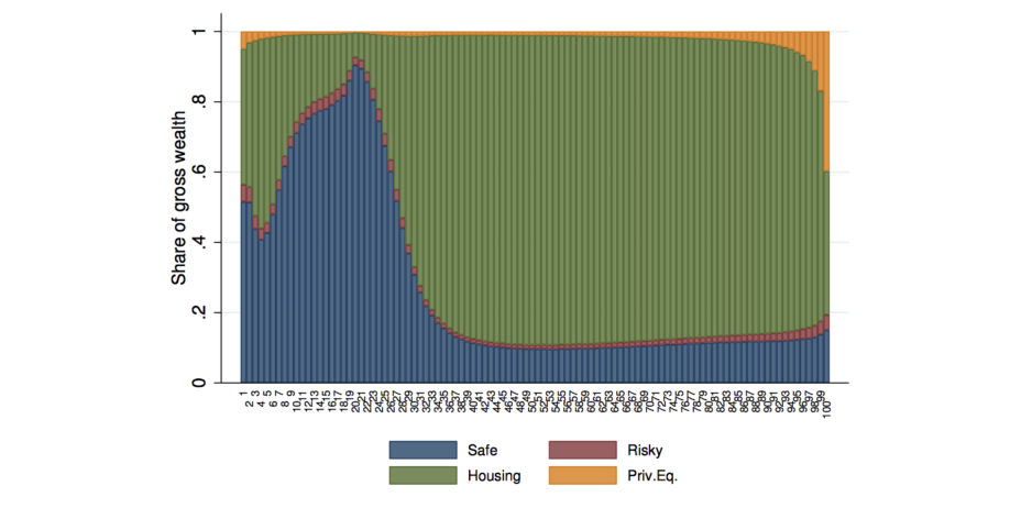
Example: share of wealth to risy asset over wealth percentiles (Fagerend, Andreas et al: "Heterogeneity and persistence in return to wealth").
Intuition:
- it is common discussion that wealthier people are willing to bear more risk than poorer people
- this is often complemented by a stronger assumption: non-increasing (or decreasing) relative risk aversion.
Impact of a change in risk
Should the demand for a risky asset increase or decrease with the riskiness of such an asset?
PropositionA shift of the distribution of returns increases the demand for the risky asset is:
- the shift is first-order stochastically dominant and for all .
- the shift is second-order stochastically dominant and for all , relative risk aversion is increasing and absolute risk aversion is decreasing.
7. Risk sharing and insurance
We consider a single good and two dates:
- : where the contingent exchange contracts are signed
- : where the contracts are settled.
We now consider a probability space, , with is a state of the world.
is the known probability distribution on if state of the world occurs, a total amount of resources is shared across agents.
There is a infite number of agents. They have NVM preferences and are risk averse.
The utility of agent is denoted as and satisfites the Inada Condition:
An allocation with is the specification of a contingent consumption plan for all the individuals in each state of the world.
An allocation is feasible if in each state the total consumption equals the total resources:
An allocation is Pareto Optimal if it is a feasible and if there is no other feasible allocation such that, :
with at least one strict inequality.
Mutuality Principle Proposition (Borch)
If all agents are strictly risk averse and have identical beliefs (same information), then for any Pareto-optimal alllocation:
Let's then proceed with the following example.
Consider the matrix of state-contingent consumption, where lines corresponds to individuals and column to states of the world:
In this case, the matrix is not a Pareto Optimal allocation.
The columns represent the aggregate resources by state:
State 4 and 5 have the same aggregate resources: , but the Borch condition is not satisfied: .
Optimal allocation: Characterization
Theorem
A feasible allocation such that is Pareto optimal there are nonnegative weights and such tat and :
This condition can be restated as:
- the ratio of marginal utilities in a given state for 2 agents is independent of the state :
- the ratio of margina utilities in 2 given state is the same across all agents:
Assume that all agents are risk averse. Then, for any Pareto-optimal allocation, and are comonotonic:
Intuition: is about the aggregate risk (how much total output/income the economy has in each scenario, is about risk sharing, who beras how much risk across scenarios).
Since , the variables are also comonotonic.
ProofAssume that the allocation is Pareto optimal. Then and the ratio is independent of . Hence the cariables are comonotonic:
Let's proceed with an example. Consider the following matrix where lines correspond to individuals and columns to states of the world:
In this case, we have resources equal to:
To check if it is Pareto-optimal for risk averse individuals (not necessarily with the same preferences), we check the commonoticity with aggregate endowment/resources: when is higher, also each should be weakly higher.
We order the states by , and we see that each row follows the same order for each agent, resulting then in a Pareto-optimal allocation:
- agent 1:
- agent 2:
- agent 3:
If the agents have same preferences, we need to check the condition:
But in states 1–4, , so the ratio must be . Then in state 5 you would need , impossible with strictly decreasing (strictly risk-averse )
Risk neutral agents should bear all the risk
Corollary
Assume that there is a risk-neutral agent and that the allocation is pareto-optimal. If agent is strictly risk-averse, then her consumption must be determnistic:
In other words: for a risk-averse agent, the consumption is independent of the state of the world .
An example of Pareto-optimal allocation - CARA preferences
Assume . Them we have:
For an allocatio to be optimal, the ratio has to be independent of , that means:
that, if we assume , implies:
If we denote by the absolute risk tolerance of and the aggregate absolute risk tolerance, summing over and using the feasibility condition gives:
and thus
Taking the expectation under the distribution of gives:
(Note that , the value taken in state is not random).
- All Pareto-optima assume that the allocation is the same. Agent takes of the aggregate risk, where is, again, the absolute risk tolerance.
- Aggregate risk is therefore spread over all the agents, but the more risk averge agent take less risk.
- The difference between different Pareto-optimal equilibria is only reflected in the levels of expected consumption .
Risk Sharing Equilibrium
Suppose there are agents with strictly concave utilities, each with endowment . Suppose that there' a complete market .
An equilibrium is given by a state price vector and a consumption plan such that:
- for all (scarcity constraint of feasibility)
- each agent's consumption plan is optimal, i.e. solves:
Intuition: agents trade claims so that consumption is moved from states where they are relatively well off to states where they are relatively poorly off.
Economically speaking, is the today-price of getting 1 unit of consumption only in state (market-insurance price of the future state).
If we denote by the Lagrange multiplier associated with investor 's budget constraint, the first order condition for the individual utility maximization is:
Intuition: at the optimum, the marginal utility of consumption in each state, weighted by its probability, equals the its price.
which implies that any equilibrium allocation is necessarily Pareto-optimal.
Risk Sharing Equilibrium - TheoremFor any initial endowment , there exists a competitive equilibrium supported by some prices . This equilibrium is Pareto-Optimal.
Intuition: if all claims can be traded, then a competitive equilibrium exists and it is efficient.
Financially speaking, this is the model behind insurance and asset pricing: markets aggregate beliefs and redistribute risk implementing the best feasible risk sharing given the initial resources and preferences.
8. Mean variance analysis
Mean-variance analysis was proposed independetly in 1952 by Harry Markowitz.
For his research, Markowitz was awarded with the Nodel Price, along with Sharpe.
The main assumptions are that preferences over portfolios are:
- increasing with respect to expected return (reward)
- decreasing with respect to variance (risK)
The basic idea of the optimization is that, given returns, variance is minimized and reciprocally, given variance, return is maimized. This leaves one free parameter, that is the agent's risk aversion parameter, which determines their choice upon the risk/reward tradeoff.
In other words, given some assets agents are assumed to maximize expected returns while keeping the variance at the desired level, or the opposite way, minimize the variance for a desired expected return.
But why do we care for mean and variance only? Results can be shown to be independent from higher moments in 2 specific cases:
- Agents have a quadratic utility index: with
- Agents have a CARA utility index and returns are normally distributed: :
We consider a probability space , is a state of the world with probability .
Any random variable defined on iss denoned with a tilde .
- takes the value in a state , hence:
- the expected value of is .
We denote by the random payoff of asset and by its price
Whem it exists, we shall denote by the safe asset, bringing a costant payoff in every state.
- By convention, the Latin subscript of denotes the risky assets . When we mean all assets, including the riskless one, we use the Greek subscript .
We call the composition of an investor's portfolio and the initial wealth, Note that short positions are possible, so we can have for some assets.
Moreover, we denote by:
-
: gross return of asset , where
-
: expected return of asset .
-
covariance between returns of assets and .
-
the covariance matrix of asset returns.
-
share of initial wealth invested in asset .
The expected return of the portfolio is given by:
Or, in matrix form as:
The variance of the portfolio is given by:
Example with 2 stocksAssume an investor has allocated her wealth equally between two stocks, .
Suppose also that , , and .
The expected return of the portfolio is given by:
and the variance by:
Note that in the same formulation sometimes we use correlation coefficient .
Minimum variance portfolio with two stocks
Given , the investor choose to minimize the variance of the portfolio:
If we apply the first order condition:
(assuming or ).
If we plug the solution into the formula for the variance of the portfolio we get:
We can then see two special cases:
- :
- :
and we can do the following remarks:
- with assets with identical variances and that are indepedent, the optimal minimum variance portfolio is such that the same amount is invested in each stock: . This is the idea behind diversification.
- with perfectly negative correlated stocks, we can obtain a portfolio with no risk.
Efficient frontier, no safe asset
In the general case, the problem for the investor is to minimize the variance of the portfolio for a given expected return .
The problem writes as:
(assuming no redundant asset)
In matrix form:
where is the covariance matrix and is the vector of expected asset returns.
(assuming no redundant asset)
Let's now denote by and the Lagrange multipliers for the constraints and write the Lagrangian:
By FOC (note: appears in the sum when and when )
If we denote by the inverse of the covariance matrix :
If we plug this into the two constraints we get:
or, in compact notation:
A solution for this system is given by:
Pre-multiplying the FOC of the problem by yields:
or, equivalently:
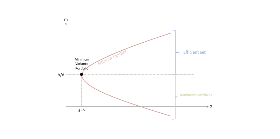
The global minimum variance portfolio (hedging portfolio) is the portfolio with the smallest variance. This portfolio (obtained with ) is given by:
It has expected return and risk .
Note that portfolio on the efficient frontier with are dominated, since one can get higher returns with the same variance.
The Mutual Fund Theorem I (no safe asset)
Given two frontier portfolios , all efficient portfolios can be obtained by mixing . Thus all agents seeking for frontier portfolios need only to invest in a combination of these two funds.
Every efficient portfolio is characterized by a scalar such that:
So, given two portfolios with return , alows to move along the efficient frontier:
Efficient Portfolio with a Safe Asset
We now consider the case of a portfolio with one safe asset and risky assets.
The investor goal is to optimize:
The FOC are:
Subtracting the two equations removes and gives:
so the risky portfolio is chosen to match the vector of excess returns .
We then put and calculate :
This means each risky weight is proportional to a weighted combination of excess returns, where the weights come from the inverse covariance matrix. Intuition: assets with higher expected excess return get more weight, but assets are also penalized if they are highly risky or strongly correlated with other risky assets.
We can see that for any efficient portfolio, the risky-asset sub-portfolio is proportional to .
We then define the tangent portfolio as the only efficient portfolio which does not use the safe assets, such that and, we have:
Once we define the tangent portfolio and a risk-free asset exists, all efficient portfolios are built in the same way combining a common risky portfolio (tangent portfolio) and some amount of the same asset.
So the tangent portfolio is the unique risky-only efficient portfolio. It is “special” because every other efficient portfolio has the same risky-asset mix, just scaled up or down.
In formulas, we write:
where is the portfolio composed of the risk-free asset only and is the tangent portfolio (with no investment in the risk-free asset).
To choose , we consider the desired return and variance:
The Mutual Fund Theorem II
In the presence of a safe asset, efficient portfolios are a combination of the risk-free asset and the tangent portfolio. The exact combination is determined by .
CorollaryAll efficient portfolios are on a real line in the plane and this line is called the capital allocation line.
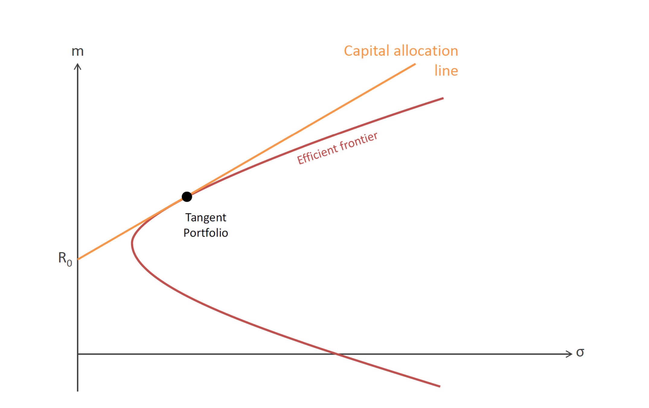
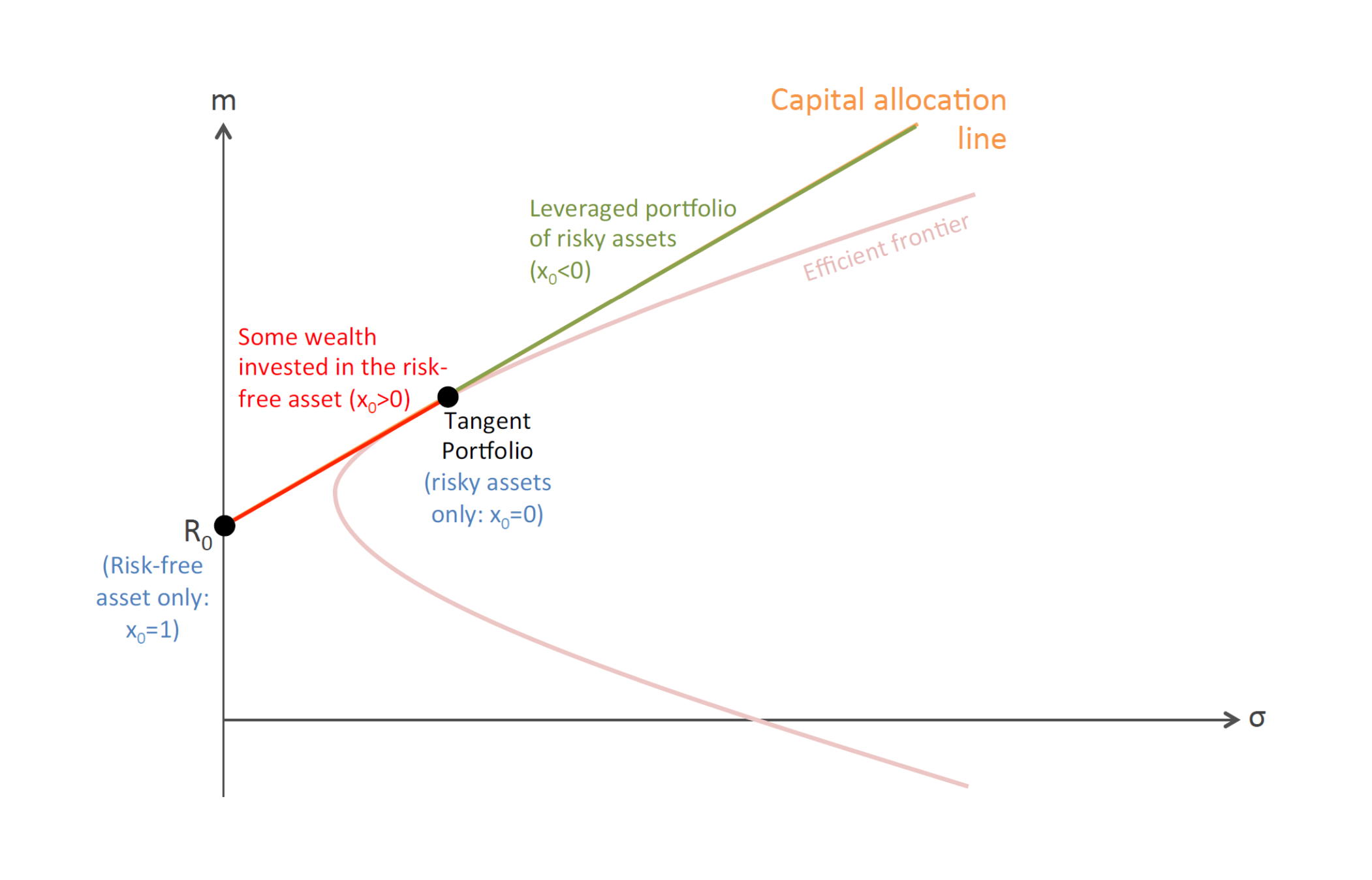
Intuition: in a economy with only risk-assets, all the efficient portfolios lie on the efficient frontier curve. If instead in the economy there exists a risk-free asset, the efficient frontier collapses into the capital allocation line (any efficient portfolio in that case lie on the straight line).
With a combination of a safe portfolio and a risky portfolio, investors can improve and expand the set of opportunities available from the efficient frontier:
- all portfolios on the capital allocation line offer a better expected return than risky portfolios with the same volatility located on the EF.
- borrowing at the risk-free rate to get additional funds allows investors to seek higher expected returns (higher ) and assume more risk (higher ).
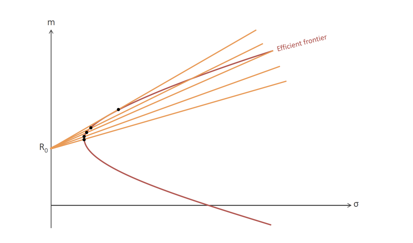
Sharpe Ratio
For any portfolio with expected return and standard deviation we define the Sharpe ratio as:
Intuition: it quantifies the performance of a portfolio measuring the excess return per unit of risk (deviation). The slopes of the drawn lines are equal to the Sharpe Ratio of the portfolios located on the EF.
- the tangent portfolio has the highest Sharpe ratio among portfolios of only risky assets.
- all efficient portfolios have the same Sharpe ratio equaling the one of the tangent portfolio.
- the slope of the capital allocation line is equal to that Sharpe ratio.
9. CAPM
The CAPM (Capital Asset Pricing Model) was independently introduced by Treynor, Sharpe, Lintner and Mossin in the 1960's.
The motivation of their works was to address criticisms of Markowitz's MVA, some of them were:
- MVA requires the full knowledge of the returns' correlation, which grows quadratically with the number of assets
- even if robust estimation of are available, MVA makes global predictions ignoring the information present in the market.
The CAPM brings two key assumptions added to the Markowitz model:
- complete agreement on the joint distribution of asset returns
- borrowing and lending at a risk-free rate available to all investors.
Under these assumptions, all investors see the same opportunity set and hold the same tangent portfolio of risky assets, which is therefore the value-weight market portfolio.
The CAPM rests on the notion of market portfolio, which is simply the aggregation of the economy's financial assets. Therefore, a fundamental assumption of the CAPM is that the market portfolio is efficient in the sense of Markowitz and this implies that all investors know the Capital Allocation Line which can be read in the market.
We now define the market portfolio as as the portfolio of all assets in the economy.
, the share of wealth in asset (market weight)is given by:
The market portfolio is assumed to be efficient, so, by the mutual fund theorem, we have:
The gross return of the market portfolio is determined by the weighted average of the asset returns as:
If we now recall that :
If we then put we get:
and multiplying both sides by and summing we get:
or, in other terms:
if we substitute out (the Lagrange multiplier from the mean-variance optimization that links covariance to excess returns), we get the very famous CAPM relation:
The CAPM tells us that the risk premium associated to asset is given by the product of the asset's beta with the risk premium of the market portfolio.
- we call idiosyncratic a risk which has zero correlation with the market. According to CAPM, idiosyncratic risk has zero premium. (This doesn't mean that this risk is liked by all investors, it just means that there is zero net supply/demand in the economy for that risk)
- in equilibrium, no agent bears any idiosyncratic risk as every agent has a combination of the market portfolio and the safe asset
On the other hand, we call systematic a risk which has correlation to the market risk and cannot be avoided by investing in the market.
- the CAPM shows that, for the same expected value, assets which are negatively correlated with the market have a greater price (and thus lower expected returns). there's net demand for those assets in the economy as they insure the investors against systematic risk
- assets which are positively correlated with the market are in net supply: people dislike them as they increase systematic risk, so they ask for an higher risk premium.
Empirical Application - Tests on the cross-section of stock returns
Empirical strategy:
- choose a benchmark (S&P500)
- compute expected returns of each individual asset
- compute all covariances between the asset and the index
- compute the variance of the index
- compute
- regress a cross-section of average asset returns on estimates of asset betas
The CAPM should then predict:
- intercept will be the risk-free rate
- coefficient on is the expected excess return of the market portfolio
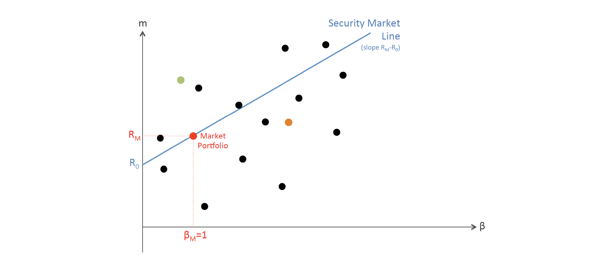
(Each data point represents one asset)
The regression line is called the security market line, its origin is the risk-free rate.
- any asset on the security line is fairly prices
- any asset under the line is overprice
- any asset over the line is underprice
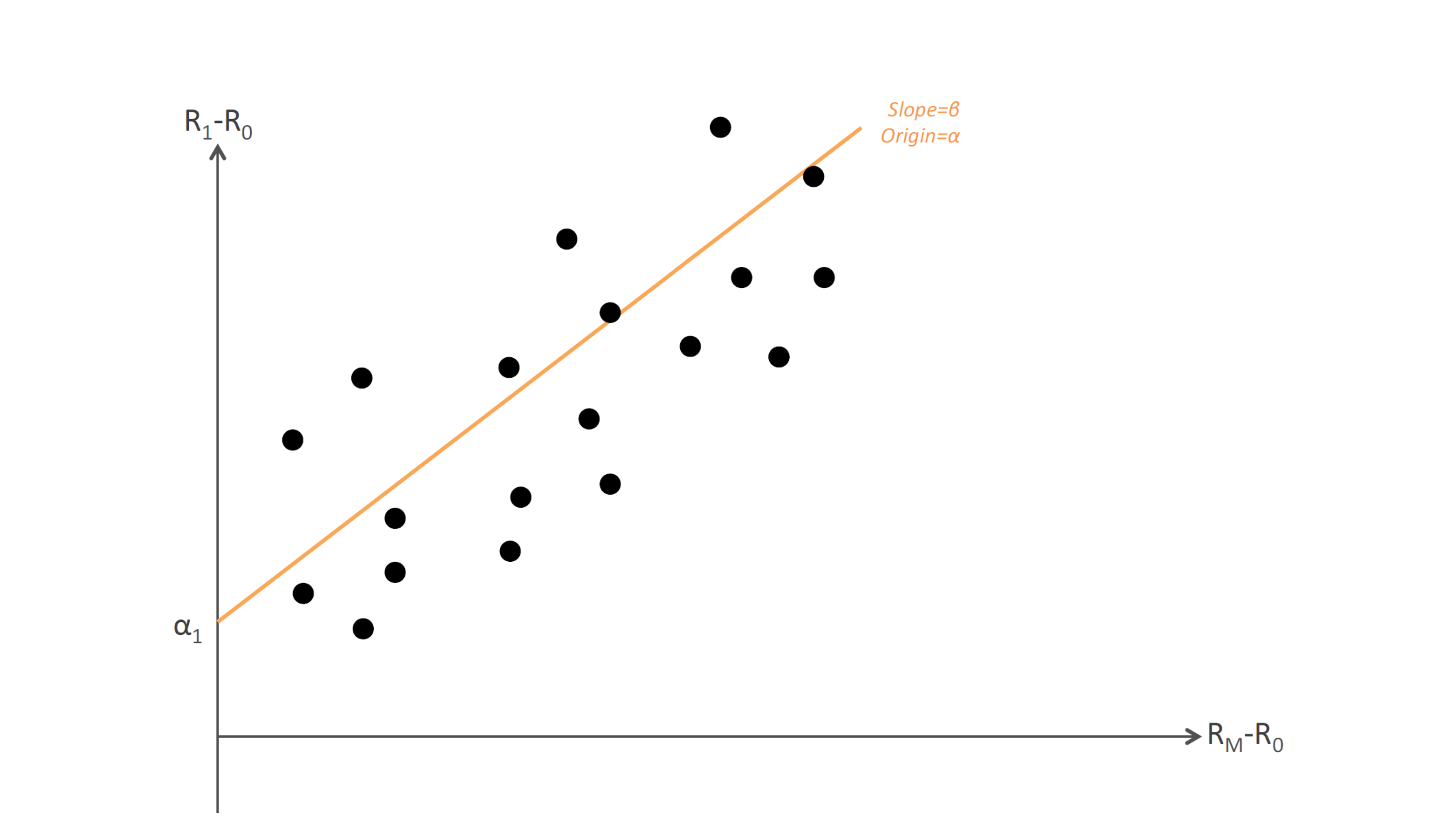
Time-series regression tests
According to CAPM, the expected value on an asset's excess return is completely explaine by its expected CAPM risk premium .
This suggests estimating the following-time series regression:
where the regression constant is called Jensen's alphak$.
- theory predicts , but empirical finance has spent the last 40 years looking for positive alpha
- those correspond to underpriced assets as the investors are expecting a greate return for the same beta.
- these assets represent arbitrage opportunities.
- Positive and significant slope for the Security Market Line
- The relation between beta and average return is much flatter than CAPM predicts
- Other variables (price ratios, size, momentum) are significant predicors of average returns Fama and Frech 5 Factors Model
The CAPM has indeed not ben an empirical sucess, raising questions about its use inm appications. Some possible explanations:
- the market proxy problem:
- empirical tests use proxies of the market portfolio
- the market portfolio at the center of the teory is not observable CAPM has never been really tested
- the CAPM relies on strong and unrealistic assumptions: need to develop more sophisticated asset pricing models (example Consumption Based CAPM)
10. Risk sharing and asset prices in a market equilibrium (CCAPM)
The Consumption Based CAPMWe consider a probability space , where is a state of the world with probability .
We denote by any random variable define on . We say that takes the value in state and its expected value if .
We consider then agents living in two periods. For each agent :
- at : deterministic endowment with consumption
- at random endowment with consumption
We write .
Agents are expected utility maximizers with additively sperable utility function:
where denotes the time preference.
We then consider a market with risky assets where is the random payoff of asset with price .
There's also a risk-free asset yielding a costant payoff for every state.
We then define by: .
Agents' optimization problemAgent maximizes his utility function, that means:
under the budget costraints:
Intuition: the first constraint represents current consumption as the initial endowment, minus the cost of investing in the risk-free asset (discounted at rate ) and the cost of investing in each risky asset .
The second budget constraint represents that future consumption is equal to the sum of the future endowment, the return of the risk-free asset and the returns from risky assets.
We can then substitute in the utility formula and we get:
We apply the first-order conditions (FOC) with respect to every choice variable :
that brings to:
Intuition: the first equation describes the trade-off between current and future consumption, incorporating the risk-free interest rate and time preference
The second equation represents the optimal condition for risky asset allocation, since it equates the marginal cost of investing in risky asset to the discounted expected marginal utility of the returns.
More explicitly, the derivation is just the chain rule:
- when increases by one unit, current consumption falls by and future consumption rises by one unit in every state;
- when increases by one unit, current consumption falls by and future consumption in state rises by .
So the two FOCs are:
The first one tells you how much current consumption the agent is willing to sacrifice for a risk-free payoff tomorrow. The second one says that, at the optimum, the price of a risky asset must equal the discounted expected marginal utility value of its payoff.
They can be combined as:
We now focus on the case linear, that means: .
We then get:
If we plug the covariance in the FOC we obtain:
We now model the consumption as:
we then denote by the variance-covarianc matrix of and we get, in matrix notation:
We then define by the absolute risk tolerance for investor :
If is linear we have:
so the previous equation rewrites as:
Market ClearingThe accounting balance is , this implies that in all states of the world:
Intuition: the total consumption in any state of the world cannot exceed the total resources (endowments) available in that state.
We now sum over all individuals and we get:
Aggregate risk-toleranceWe define by the aggregate risk tolerance as:
Then if we use and in every state we get:
If we isolate we obtain the Consumption Based Capital Asset Pricing Model (CCAPM):
In the CCAPM we can decompose the price of a risky security as the sum of:
- the discounted expected value of its payoff
- minus a risk-premium that is proportional to the correlation between the security's payoff and the aggregat risk:
Important: the CCAPM is more general than the CAPM it's explicitly derived from a market equilibrium.
The CCAPM links the price of securities to underlying movements in the fundamental characteristics of the economy (macroeconomic fluctuations in aggregate consumption or income).
Interpretation of the CCAPM
According to CCAPM, the expected return of an asset is equal to the risk-free rate if its payoff is uncorrelated with the aggregate risk in the economy.
Like in the CAPM, the risk-premium can be positive/negative depending on the sign of the correlation:
- a positive correlation between the security and the aggregate risk lowers the security price
- note that the aggregate/total endowment in the economy represents the risk/uncertainty in the econommy when the economy is doing poorly, people value consumption more
- the security's payoff is high when the economy is doing well and the opposite the security is less desiderable because it doesn't provide insurance against bad states of the world the investors require higher risk-premium to hold this security
- a security that shows a negative correlation with the aggregate risk can be then used to hedge against macroeconomic risk the price of the security will be higher.
The risk-free rate
Under CARA and preferences and Gaussian risks, the risk free rate of interest:
- decreases with (impatience effect)
- increases with (average endowment effect)
- decreases with risk (precautionary savings effect)
More on the CCAPM (Videolecture)