The following notes come from the course Economic Growth, Cycles and Policy, held by Prof. Dr. Hans Gersbach at ETH Zurich.
(I spent one semester working for Hans Gersbach at KOF and I couldn't be more enthusiastic: he’s clever, prepared, and very inspiring.)
Please refer to his list of publications to deep dive in the subject.
Index
- Introduction
- Macroeconomic Schools
- IS-LM Model in Closed Economy
- Aggregate Demand and Aggregate Supply Curves
- Control of Interest Rates and Taylor Rule
- Schools of Thought
- Consumption and investment
- The Solow Growth Model
- Money holding: Inflation and Monetary Policy
- IS-LM Model and Open Economy
- Bank Runs and The Diamond-Dybvig Model
- Crises in Market Economies
- Macroeconomic Forecasting
1.1 Introduction
Macroeconomics tries to answer some key questions:
- What determines key macroeconomic variables? (GDP, unemployment, inflation, credit, consumption, interest rate...)
- How can economic policy influence these variables? (government spending, tax policies, monetary policy, "wage policy"...)
- How can macroeconomic policy and market regulation operate together?
- Do macroeconomic processes show inherent dynamics? (cycles, trend and instabilities)
- Should economic policy focus mainly on long-run growth or on stabilization of the business cycle?
To start answering them, we firstly start with some stylized facts of Macroeconomics:
Note that, if a variable is procyclical, it moves in the same direction as the overall economy.
| Economic Variable | Cyclical Behavior | Timing & Characteristics |
|---|---|---|
| Output Growth | Procyclical | Highly correlated across all sectors |
| Consumption & Investment | Procyclical | Investment is significantly more volatile than consumption |
| Employment | Procyclical | Unemployment is anti-cyclical (moves in the opposite direction) |
| Real Wages & Labor Productivity | Procyclical | - |
| Money Supply & Stock Prices | Procyclical | React early in the cycle (Leading indicators) |
| Inflation & Price Level | Procyclical | React delayed in the cycle (Lagging indicators) |
| Nominal Interest Rates | Procyclical | React delayed in the cycle |
| Bank Credit | Procyclical | - |
| Government Spending | Procyclical | Usually follows the direction of the cycle |
Some additional common rules of macroeconomic policy, based on consensus, argue that:
- in case of liquidity problems, the central bank should provide liquidity by raising money supply.
- government spending and investments of infrastructure should not be lowered during recession periods.
- in downturns automatic stabilizers (first responders to an economic crisis) should work.
- in the long run monetary policy has to focus on price stability (inflation around 2% a year).
- real wage increases should not exceed productivity growth when at the same time the number of employees remain constant.
1.2 Macroeconomic Schools
The following graph shows the evolution of the macroeconomic thought from 1950 till today.
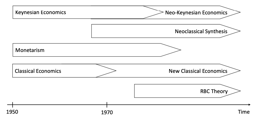
The Keynesian Branch
- Keynesians: focus on the short-run. They argue that markets don't always clear and that government intervention is necessary to manage the business cycle.
- New Keynesians: they introduce microfoundations (explaining how people behave and spend) and nominal rigidities (prices and wages don't adjust instantly, which justifies government intervention).
The Classical Branch
- Classical: they argue that markets are self-correcting and the invisible hand ensures optimal employment in the long run.
- New Classical: emerged in 1970, they introduced rational expectations, suggesting that because people anticipate government policy, those policies often become ineffective.
The Monetarist & RBC Branch
- Monetarists: led by Milton Friedman, they argued that changes in the money supply are the main driver of economic fluctuations.
- RBC Economics (Real Business Cycle): they are a subset of New Classical thought. They argue that "cycles" aren't failures of the market, but rather efficient responses to technological shocks or changes in productivity.
Economic Schools of Thought: Crash Course Economics [Video]
Classical v. Keynesian Theories [Video]
2.1. IS-LM Model in Closed Economy
In the long run:
- prices are flexible
- output is determined by factors of production and technology
- unemployment equals its natural rate
In the short run (IS-LM setting):
- prices are fixed (or change slowly)
- output is determined by aggregate demand
The IS-LM Model [Wikipedia]
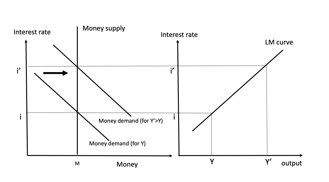
The LM-curve (positive relationship between real interest rate and output)
In equilibrium, money supply equals money demand:
where is a function representing the liquidity preferences, is the interest rate and the price level.
If we consider:
where:
- : Sensitivity of money demand to changes in income ().
- : Sensitivity of money demand to changes in the interest rate ().
If we write and solve for :
This yields an upward-sloping LM curve, which represents the positive relation between the interest rate and the output.
In this model:
- the Central Bank (CB) controls money supply
- if output increases, the demand for money increases at any .
- for a fixed supply of money, must increase to lower the demand for money and maintain equilibrium.
It is also important to distinguish between:
- Movements along the curve: caused by a change in output ().
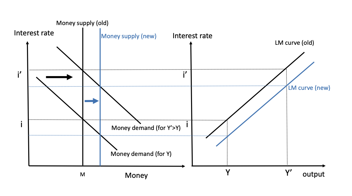
- Shifts of the curve: caused by changes in Monetary Policy (the Money Supply).
Indeed, increasing money supply leads to:
- increase in demand for money to maintain equilibrium must decrease
- for any level of output , the corresponding is lower.
The result is that an increase in the money supply leads the LM curve to shift down:
- or, equivalently:
- or, equivalently: .
The IS-curve (negative relation between real interest rate and output)
Assumptions:
- there is only one good that can be used for consumption or investment
- all demanded goods will be supplied (no rationing of demand).
We then model planned expenditures :
where is the consumption, physical investments (not financials!) and the public spending.
When planned and effective expenditures are equal and we obtain the IS-curve.
If we consider: , we obtain the following:
Even though the IS-curve is often referred to as the goods market equilibrium condition, this is misleading.
In microeconomics, a market equilibrium balances demand and supply via price adjustments (market clearing condition).
The IS-curve does not reflect endogenous price levels.
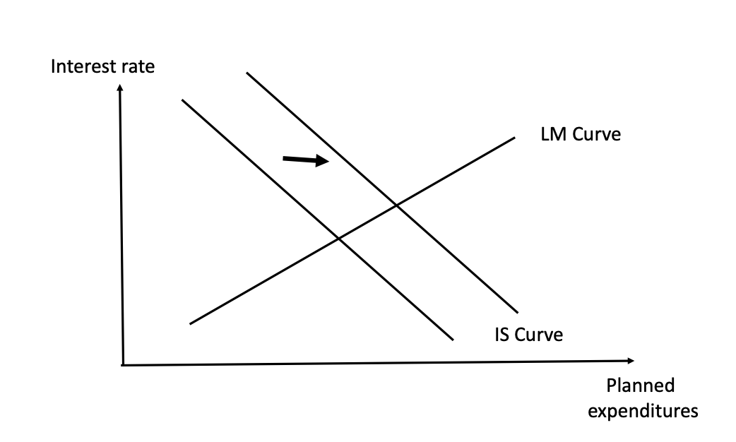
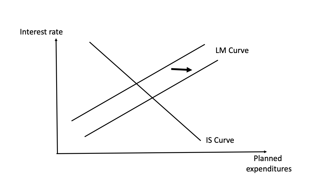
The Multiplier-Process in IS-LM Model
Intuitively, if we consider an increase in public spending :
- increase in public spending moves the IS-curve to the right, increases.
- the LM-curve remains unchanged
- in the short run, interest rate and output increase.
In formulas, if we consider and we solve both IS and LM equations simultaneously, from the LM-curve we get:
if we substitute this into the IS-expression:
If we consider or, equivalently, we take its partial derivative:
Dividing both sides gives us the Fiscal Policy Multiplier:
- : represents the how much goes into savings (smaller this is, the bigger the multiplier).
- : is the monetary drag.
- If is high, income growth creates massive money demand.
- If is high, investment is very sensitive to interest rates.
- If is low, it takes a larger increase in to balance the money market.
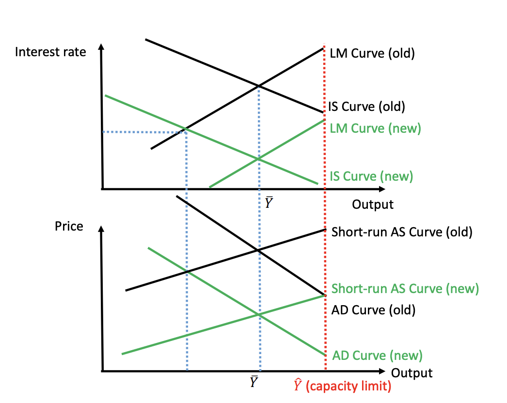
Easing of monetary policy
- Central Bank increases money supply by setting lower interest rate at given .
- The LM-curve shifts downward
- The IS-curve remains unchanged
- increases (with unchanged because exogenous, increases and increases) and declines
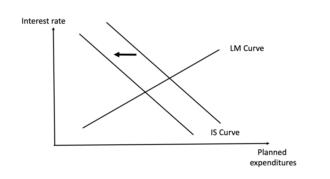
Declining consumer confidence
- It may be caused by financial crisis, wars, terror attacks or whatever
- Households consume less and save more of given income
- the IS-curve shifts leftward
- LM-curve remains unchanged assuming, for simplicity, that the demand for money does not change
- and decline.
Possible counter-measures to stabilize :
- Expansive fiscal policy can shift the IS-curve to initial position
- Easing of monetary policy implies downward shift of LM-curve
2.2. Aggregate Demand and Aggregate Supply Curves
So far we've been using the IS-LM model to analyze the short-run dynamics. However, a change in price level would shift the LM-curve and therefore affects the output.
The (aggregate demand) AD-curve describes the relationship between price and output.
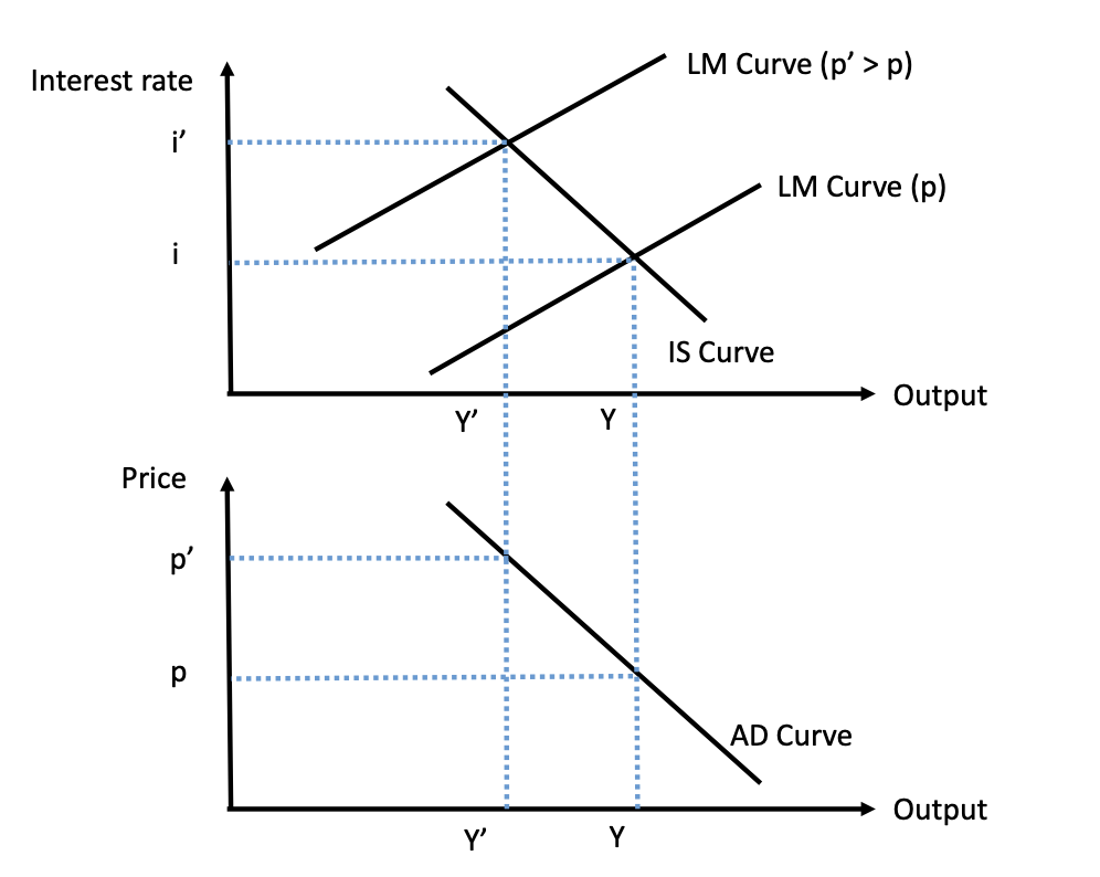
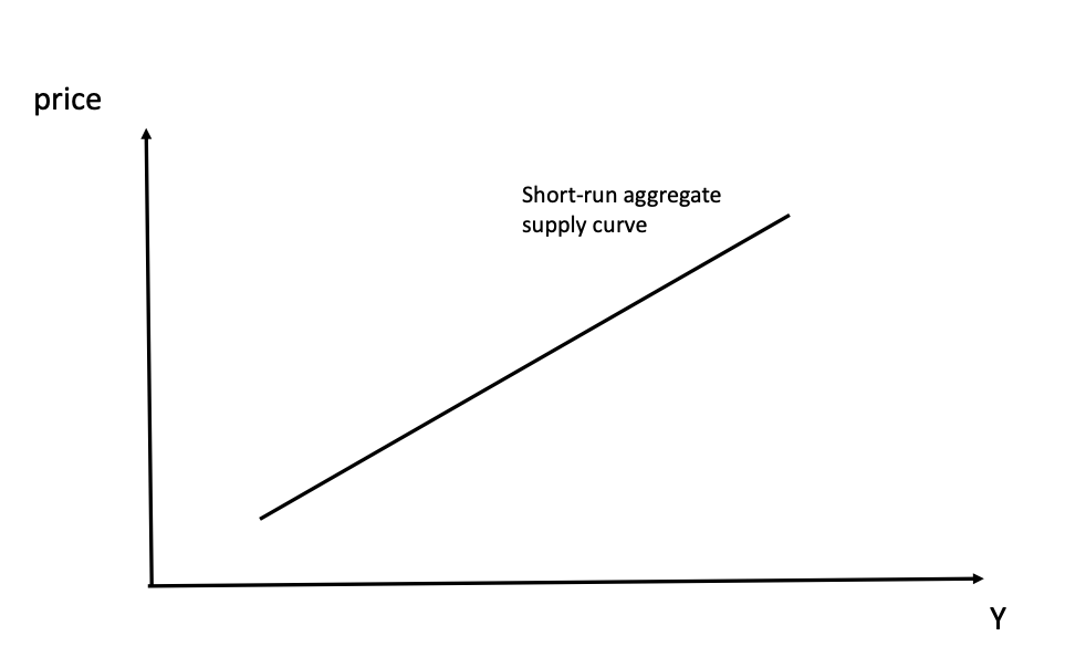
On the other hand, we can model the short-run aggregate supply curve with an upward slope (given by sticky wages and sticky costs).
We now give an example of complete adjustment and we see what happened with a reduction of the government spending.
Firstly, a reduction in shifts both IS and LM-curves left.
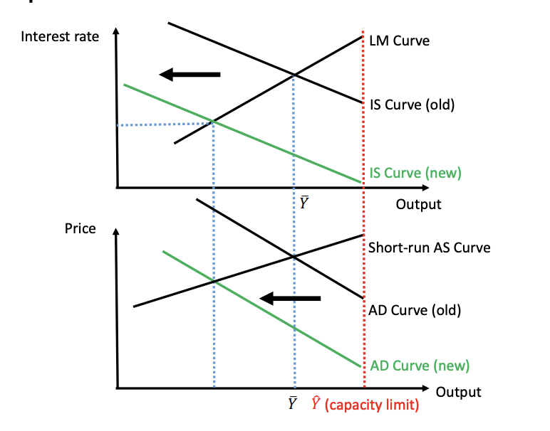
In the short-run equilibrium, is lower than the initial-natural value .
Therefore, aggregate supply moves down and we see a gradual adjustment of prices, leading to a downward-shift of the LM-curve that, finally, brings the system back to .
In reality, downward price and wage adjustments are difficult (see for example, the Greek crisis in 2010-2016):
- very long wage contract make them hard to re-negotiate
- resistance of particular groups of employees.
In the case of Greece:
- costs were also partly determined by international markets due to imports
- governments had to rely too much on increasing value-added taxes that led to an increase in prices.
2.3. Control of Interest Rates and Taylor Rule
Models with LM-curve assume that the CB uses the money supply as an instrument, therefore will be determined endogenously by the equilibrium.
In reality, CB uses short-term interest rates as their policy instruments (rather than the money supply).
The main advantage of targeting interest rates versus money supply is that, in the second case, the difference between fluctuating demand and stable supply would lead to strongly fluctuating interest rates.
Nowadays CB counterbalance fluctuations in money demand by adapting the money supply to maintain the short-term interest rate at the targeted level.
CB influences short-term interest rates .
- A risk-neutral investor must be indifferent between:
- make a long-term investment with interest rate
- make short-term investments in each period at interest rate (with denoting the expected interest rate)
But, in practice:
where denotes the positive term premium associated to the uncertainty of the future rates and the risk of refinancing.
In this way, by influencing the short-term nominal interest rates, the CB can also influence the long-term ones.
3. Schools of Thought
Real Business Cycle (RBC) Theory
The following basic RBC-model starts with the following assumptions:
- an infinitely long-living household/agent maximizes the expected value of
with respect to the intertemporal budget restriction, where represents the utility in period and the discount factor.
- a representative firm maximizes profits, given its production function.
- there exist no frictions (no price rigidities, no externalities, no asymmetric info, no public goods...)
The aggregate production function is then:
- aggregate output
- measure for the efficiency of labor (stochastic), example: , with , where describes the persistence of the shock.
- capital
- labor input
- share of physical capital
Intuition: the stochastic component induce business cycles.
is then a measure for the efficiency of labor over time and relative to capital. It's a catch-all variable that includes levels of health, skill, education and technological knowledge.
Welfare TheoremUnder technical assumptions - (i) local non-satiation of preferences, (ii) competitive markets with no frictions and no externalities, (iii) price-taking behaviors - any allocation that forms a competitive equilibrium is Pareto-efficient.
However, the RBC model received several critiques:
- there's no broad evidence that strong technology shocks always affect the economy
- there's no adequate explanation of lasting recessions
- in typical RBC models, employment fluctuations come from the household's intertemporal substitution of labor; empirical studies, in reality, show little evidence for that.
- RBC models do not consider monetary shocks, but only technology shocks.
- the assumption of a unique representative agent is not accurate, small heterogeneity in utilities can have a strong influence on the model.
Monetarism
Early Monetarism started around 1920 Irving Fisher applied the quantity theory of money as a tool for quantitative analysis of prices, inflation and interest rates. The key concept behind is that the amount of money circulating in an economy is the primary driver of its health, inflation, and growth.
The quantity equation is the central and formal definition of this model:
- : stock of money
- : velocity of money
- : price level
- : real GDP
Quantity Theory of Money - Fisher Equation [Video]
The Quantity Theory (coming from the Early Monetarism) is an interpretation of the previous equation that assumes that is constant: if people’s spending habits don't change, then any change in (Money) must lead to a proportional change in .
In its extreme form, it predicts the neutrality of money: an exogenous increase of the stock of money is followed by a proportional increase of the price level, without any effect on real variables like consumption, output and investment.
Recall that, the velocity of money is defined as:
It is the rate at which currency circulates through an economy. It measures the average number of times a single unit of money is spent on domestically produced goods and services within a specific period.
Milton Friedman: "Inflation is always and everywhere a monetary phenomenon"Friedman's main idea was that should not be interpreted as a rigid constant, but rather as a function of money demand, therefore as something linked with real-world variables (consumption, investment, output etc...).
Moreover, in the 1950s, Milton Friedman and Anna Schwartz argued that money might be neutral in the long run, but it has real effects in the short run.
They linked the previous crisis with their theories: before Friedman, most people thought the Great Depression was a failure of capitalism. Friedman and Schwartz proposed that it was actually a failure of the Federal Reserve because Fed didn't put money back into the system in moments of need, resulting in a strong credit crunch and deflation.
If compared with Keynesians, Monetarists show a different approach:
| Feature | Keynesian View | Monetarist View |
|---|---|---|
| Main Tool | Fiscal Policy (Spending/Taxes) | Monetary Policy (Money Supply) |
| Phillips Curve | Trade-off: You can have low unemployment if you accept higher inflation. | No long-run trade-off. Pushing inflation only works in the short-term. |
| Stability | The economy is inherently unstable. | The economy is stable if the money supply is stable. |
| Inflation | Caused by high demand/rising costs. | Inflation is always a monetary phenomenon. |
Friedman was also skeptical about discretionary policy, he proposed:
- constant-money growth rule (K-percent rule): central banks should increase annually 3% the amount of money supplied, or, in general, money supply should increase with inflation.
- avoid interest rate targeting and too low (below the natural level)
- distrust of fiscal policy: government spending "crowds out" (reduces) investment and has little impact in the long run.
However, in 1980, monetarism lost its appeal for different reasons:
- the assumption on was not realistic
- it was hard to understand the definition of money stock (cash, liquid investments, cash equivalents...?)
- money growth was not a good indicator of demand
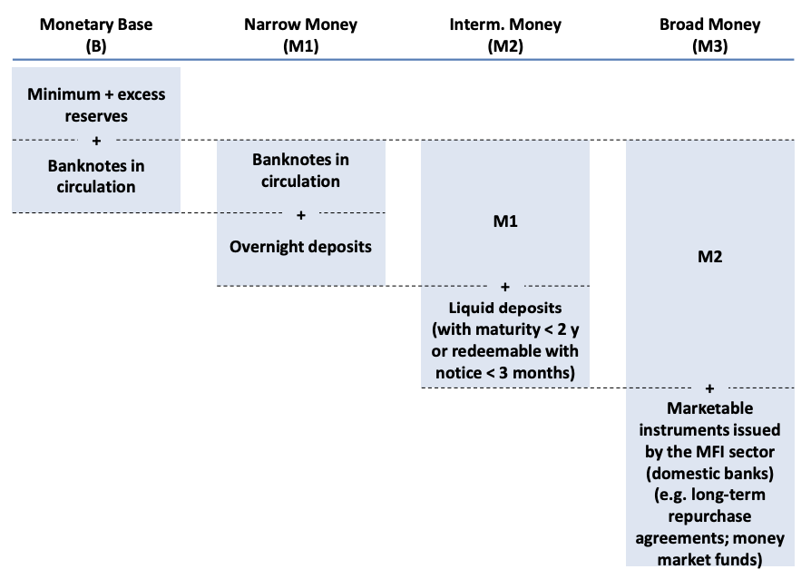
Definition of Monetary Aggregates
- M1 (Narrow Money): includes currency, i.e. banknotes, coins and balances that can be immediately converted into currency or used for payments.
- M2 (Intermediate Money): includes M1 + deposits with maturity up to 2 years and deposits redeemable with notice period up to 3 months.
- M3 (Broad money) includes M2 + marketable instruments issued by Monetary Financial Institutions.
Today's money architecture is structured as follows:
| Instrument | Issuer | Users | Role |
|---|---|---|---|
| Cash | Central bank | Everyone | Public central bank money |
| Reserves | Central bank | Banks | Interbank settlement asset |
| Deposits | Commercial banks | Households, firms | Main money in everyday payments |
Neoclassical Economics
The model, based on Lucas (1972) and Phelps (1970), starts from the following assumptions:
- the economy is populated by a large number of farmers indexed by
- each farmer produces a specific good
- each farmer sells its good in a competitive market at individual price and market price
- revenues allow each farmer to consume a bundle of goods
- there are two 2 possible shocks:
- preference shock
- monetary shock
For simplicity, we also add the assumption that there's perfect information. We then model each farmer's production as:
where is the output and his amount of labour.
The budget constraint for each individual with consumption is:
The utility function of each individual is then:
Since there's perfect information, each individual knows the aggregate price level , by substituting , each individual faces the following optimization problem:
that leads to:
if we consider and , we can rewrite the first-order condition as:
Intuition: a farmer increases his production when the relative price of his product increases.
If we then assume that the demand function depends on the good's relative price , on real income and on a real preference shock , we can write the log-demand as:
where is the elasticity of demand between goods.
Therefore, the aggregate output is given by and the aggregate price level by .
(Note that the preference shock is assumed to have zero mean: )
We then consider aggregate demand, given by: (intuition: similar to the quantity equation with ).
In log-terms, this rewrites as:
with assumed to be stochastic , representing the monetary shock (central bank's policy is unpredictable, creating random fluctuations in demand).
In this setup, the monetary shock is the unexpected realization of (i.e. an innovation in log money supply): a positive shock shifts up aggregate demand , while under perfect information it only changes in equilibrium.
In equilibrium, the market has to clear, i.e. :
solving for yields to:
if we then take the integral over all goods, we get:
Hence, this can hold if and only if , (remember that ) and .
For the individual good, this means:
Intuition:
- money is neutral and can only affect the price level, output is fixed at the full employment rate . (Classical dichotomy: monetary policy causes nominal prices and wages to change, leaving the real equilibrium unchanged).
- the equilibrium depends only on the relative price which depends on .
We now consider the same model with imperfect information, so each farmer only observes the price of his produced good but not the market price/price index .
In this way, a monetary shock has real effects on output, raising aggregate demand. As the unpredicted increase of money supply generates price movements, individuals may misinterpret this partially as an increase of relative price index of a good.
In this model, output is given by the Lucas Supply Function:
where is the slope/sensitivity parameter (how much output responds to a given price surprise), is the actual price level and is the expected aggregate price level before observing the actual price.
Intuition:
- deviation of from its natural level is an increasing function of the surprise in the price level
- if we make use of the aggregate demand function , we can solve Lucas Supply Function for and :
This model argues that there is a statistical output-inflation relation: however, if policy makers attempt to take advantage of this (raising output by raising the money growth rate above the trend level), they may cause this relationship to break down.
Furthermore, the model states that:
- the monetary shocks leads to an increase of output in the short run
- in the intermediate/long run, individuals will learn that the policy maker increases average money growth aggregate real output is no longer affected!
Lucas Critique: if policy makers attempt to take advantage of statistical relationships, the effects operating through expectations may cause relationships to break down.
However, models based on Neoclassical economy (like Lucas Supply function) are appropriate to study:
- if monetary policy has large effect if it surprises the public
- if trying to create repeatedly surprises will be futile
New Keynesian Economics
The main assumption behind is that prices are not completely flexible (Some models also consider wage rigidities).
Firm's profit maximization yields to the following New Keynesian Phillips Curve:
where represents the inflation, the output, and .
- an increasing output level leads to higher inflation
- high expected inflation tomorrow yields to higher inflation today. (If firms expect higher prices, they set higher prices today).
On the other hand, households' intertemporal consumption optimization problem yields the following IS-curve:
The IS-curve states that output depends negatively on the real interest rate and positively on the expected future output.
Also, if the real interest rate is expected to rise in the future, savings become more attractive and consumption declines.
A forward iteration of the IS-curve and the Phillips curve yields present values of expected future variables:
This forward iteration is obtained by recursive substitution of the IS relation into future expectations and by imposing a transversality condition (that expected future output does not grow unbounded), which lets us write current output and inflation as infinite discounted sums of expected future policy rates, outputs and shocks.
Intuition: firms set their nominal prices based on the expectations of future output:
- output depends on all expected future real interest rates
- inflation depends on all expected output levels.
For the analysis of the optimal monetary policy, we also add supply shocks and demand shocks , both described by an AR(1) process.
with measure the persistence of the shocks.
With demand and cost-push shocks, one common log-linear representation is:
and forward iteration yields:
Since output now also depends on expected future demand shocks, shocks on the IS side can, in principle, be fully accommodated by adjusting the policy rate path.
On the other hand, cost-push shocks (supply shocks) generate a trade-off between output and inflation ( efficient frontier).
Criticism:
- there's no delay in the response of inflation to shocks
- inflation is purely forward-looking, so past inflation is irrelevant
- in the case of demand shocks, disinflation can be achieved costlessly and may even generate a boom if anticipated. However, disinflations have historically entailed significant output losses.
4. Consumption and Investment
The Keynesian Consumption FunctionThe Keynesian consumption function has the form:
We immediately notice that consumption depends only on current income. is the constant consumption that would occur in any case.
We then define the Marginal Propensity of Consumption (MPC), that lies between and as:
Furthermore, the Average Propensity of consumption (APC), that decreases with an increasing income, is defined as:
Intuition: savings are luxuries and can only be afforded with higher income.
However, empirical observations do not prove this result: APC decreases with increasing income in the short term but, as income increases over a long-term horizon, the APC remains constant.
Furthermore, the Keynesian rule ignores expectations, wealth, credit constraints over time and life-cycle considerations.
The Life Cycle and Permanent Income Hypotheses
The Life Cycle and Permanent Income hypotheses try to solve the previous inconsistency.
The Life Cycle Hypothesis was proposed by Ando, Brumberg and Modigliani in the 1950s
The core idea is that households pursue consumption‑smoothing: they choose a consumption path that evens out spending over their lifetime (borrowing when young or low‑income, saving when earning more).
Formally, with real interest rate and a remaining horizon of periods, the household faces the present‑value (lifetime) budget constraint:
If markets allow perfect smoothing and the household chooses constant consumption for the remaining periods, then
so the constant consumption level is
Intuition: consumption depends on lifetime (present‑value) resources, not just current income; wealth typically accumulates during working years and is drawn down in retirement. Savings therefore reflect lifetime income and timing, not only current earnings.
The Permanent Income Hypothesis, proposed by Milton Friedman in 1971, states that income is a sum of permanent income and transitory income :
- Permanent income is the long-term/average income
- Transitory income is the one coming from surprises and fluctuates, with .
Consider the permanent income as your salary for your work contract, hopefully increasing with seniority; and the transitory income as some unexpected bonus, lottery wins, monetary heritage etc....
The theory suggests that, since people want to avoid fluctuations in consumption, current consumption will mainly depend on permanent income. Moreover, people will use borrowings and savings to smooth their consumption over time.
At the limit, transitory income becomes irrelevant: with .
In this model, the APC can also be expressed as:
As a result, for a given level of permament income, people with high levels of transitory income will have APCs lower than average.
Also, over the long-period, the APC should be independent of transitory income, since (shocks and fluctuations cancel each other).
According to this theory then, economic policy can affect consumption only if it affects permanent income (example: tax cuts can increase consumption only if they are not perceived as transitory).
The Fisher Approach to Life Cycle Hypothesis
We now consider a simple formal model of optimal consumption/saving.
- Consider an agent that lives for periods.
- The agent has a period utility with a discount factor with .
We also assume and . - The agents faces the following budget constraints:
- Period:
- Period: where denotes the real interest rate.
So, if we plug toghether, we end up with the following intertemporal-budget constraint:
The agent then faces the following optimization problem:
At the optimum, the Euler/Tangency condition (the point where a consumer has perfectly balanced their budget to get the maximum possible satisfaction) can be derived with the following Lagrangian:
Computing the partial derivatives with respect to gives:
Intuition:
- if : the agent should consume more on the first period and save less.
- if : the agent should shift consumption to the second period and save more. The model has then these implications:
- Consumption depends on the (expected) discounted income over both periods (in contrast with the Keynesian approach consumption depends only on current income)
- Consumption typically depend on the real interest rate (changes in lead to income and substitution effect).
Intertemporal Budget Constraint of the Government
In a 2-period model, the government levies taxes and spends in public goods (non rival and non-excludable).
- In the first period, the government can end up in a fiscal deficit (or surplus if ):
- in the second period, the government has to repay the deficit plus the interests:
If we combine the two equations, we obtain the Intertemporal Budget Constraint:
Intuition: the present value of government spending equals the present values of tax incomes.
As a consequence:
- if the government decides to lower taxes in the first period by keeping spending constant
- then, in the second period, it has to raise taxes by
- the tax cut increases the income of the households by in period 1 and decreases it in period 2 by
- lifetime income is given by , so, after the changes in taxation, it becomes:
- according to the Fisher model, in each period, the households consume the same amount as before the tax policy, since lifetime income was NOT affected.
This is called Ricardian Equivalence Theorem.
The Ricardian Equivalence Theorem in detail [Investopedia]Intuition: households have more money in the first period, but they know they will have less in the second, so they save to pay higher taxes in the future.
Despite this theorem, governments often try to stimulate consumption by reducing taxes and keeping spending constant.
These policies are NOT completely futile, since, in practice, the Ricardian Equivalent Theorem doesn't hold perfectly. (The increase in households' current income increases their consumption by some positive fraction of the additional income).
This comes from the fact that, in most cases, households are myopic: they notice an increase in income, but they are unable to predict a future increase in taxation (households are not 100% rational and follow simple rules).
However, even in theory, there are some possible deviations from the Ricardian Equivalence:
- Limited lifetime: the government can take long periods of times to repay its debt, shifting the tax burden to future generation and redistributing consumption from a generation to another.
- For this reason, if households took the utility of future generations into account, they should save more and NOT expand consumption for the expected future tax burden.
- Distortionary taxation: not always who benefit the tax reduction will also repay the tax burden (the government can levy taxes from different parts of the population)
5. The Solow Growth Model
(Productivity) growth isn't everything, but in the long run it's almost everything. Paul Krugman, 1990
Real GDP per capita is often considered the most important indicator for average standard of living.
(Is this really the case? Luciano Canova in this book answers this: is the PIL the right measure to measure happiness?)
More in detail:
- Economic growth is the increase in value of all goods and services produced by an economy. It is conventionally measured as the percent rate of increase in real gross domestic product. -- GDP is defined as the total market value of all final goods and services produced in a country in a given time period. It's defined by the National Income Identity:
The Solow Model - General Assumptions
- A closed economy (no trade)
- One good that can be consumed or used as capital
- Households save a constant exogenous fraction of their income (we are not interested in why they save , we simply put that value into the model)
- Rate of technological progress is exogenous
- No taxes, no subsidies ( no government)
- Discrete time
Output is produced according to the aggregate production function:
- : efficiency of labor
- : size of the labor force is the effective labor
- : stock of capital
Further assumptions:
- constant return to scale (CRS):
- for each argument
We model technological progress as and we consider as exogenous.
Most of the times, in the Solow Model, we assume a Cobb-Douglas production function:
(it can be easily checked that this function respects all the assumptions).
Because of the constant return to scale, the production function can be written in intensive form:
if we now introduce:
we obtain:
(This makes easier to solve the model since we only have one argument).
We now introduce some assumptions on the population growth and the technological progress:
- population (coinciding with labor force) at is
- population grows at a constant rate :
- technological level at is
- technological level grows at a constant rate :
The capital stock increases by investment and decreases by depreciation at a constant rate .
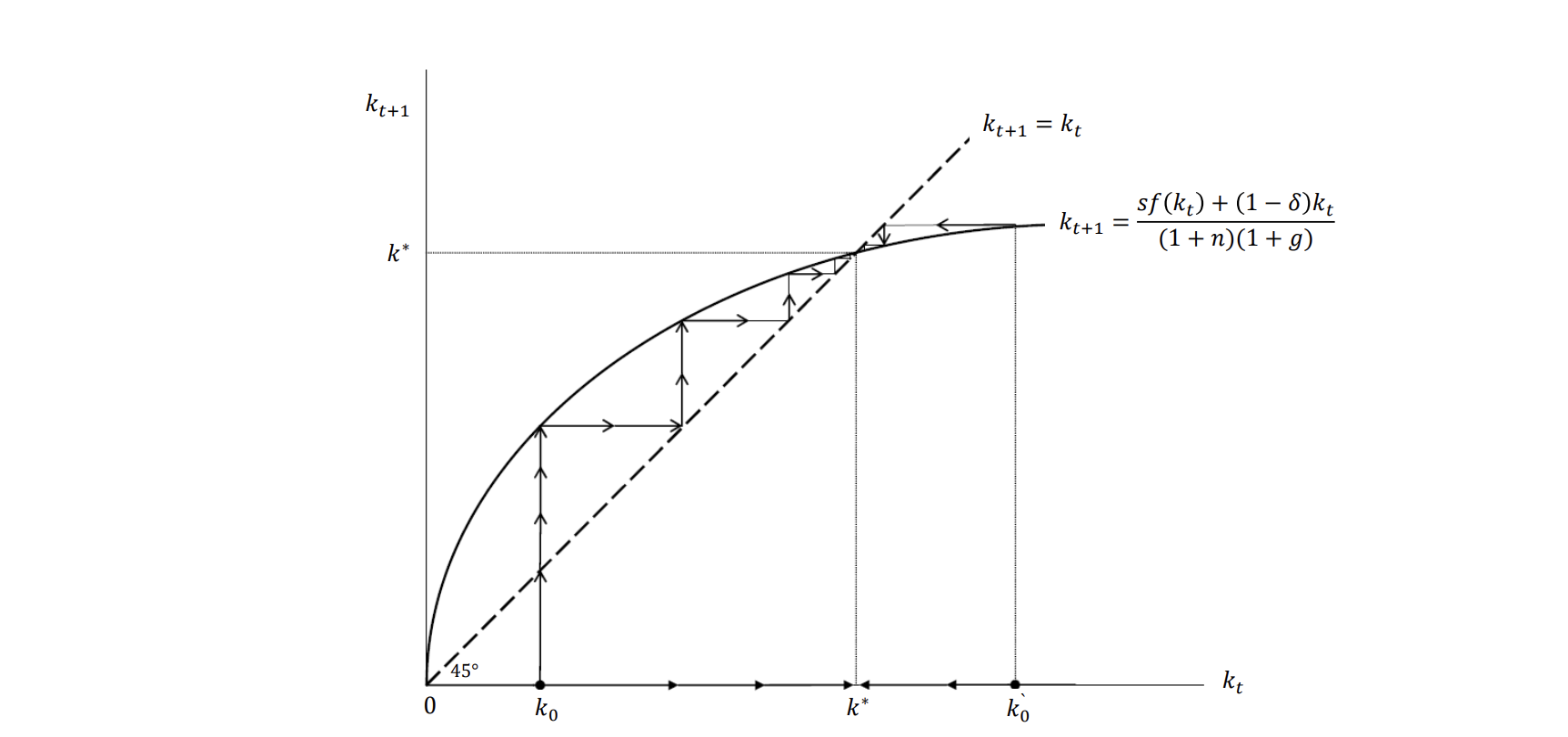
We then obtain the fundamental law of motion of the Solow Model:
In a closed economy without government spending:
If we also assume that is constant over time, this implies:
We now take some time to describe the variables. Given the ones in absolute form (, we have the Per Capita Values (simply dividing by population) as:
and the Intensive Form (simply dividing by effective labor) as:
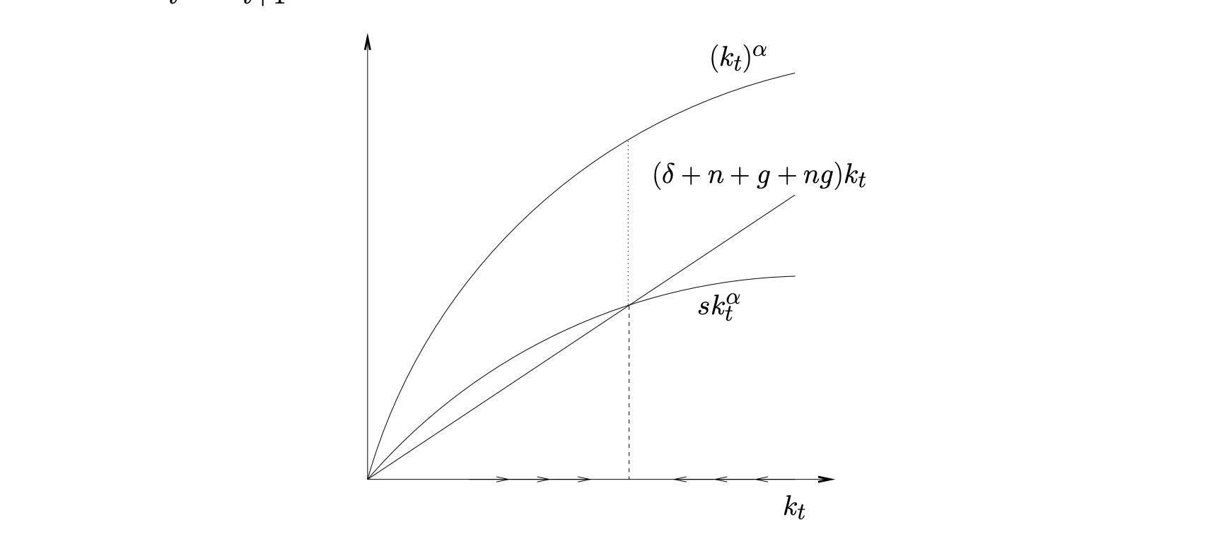
If we divide the fundamental law of motion by the effective labor too, we obtain the Capital Accumulation Equation in intensive form:
If we subtract from both sides :
Where the last equality is true if we consider the Cobb-Douglas function and it represents the Fundamental Law of motion in intensive form.
is the break-even investment (the min investment needed to prevent the capital stock in intensive form from shrinking). If actual investment is equal to the break-even investment, is constant over time.
A diminishing marginal product of capital implies that converges to where actual investment equals break-even investment.
In the long run, is constant over time, reaching a steady state
The long-run equilibrium () implies the following mathematical solution:
that brings the following properties:
- , the ratio of output for effective labor, is constant:
- is constant
- do NOT depend on the initial capital .
- Capital per capita , output per capita and consumption per capita grow at rate of technological progress:
- grow at rate for :
We can also see that changes in have only effects on per-capita steady-state values.
A change in has growth effects on per-capita steady-state values.
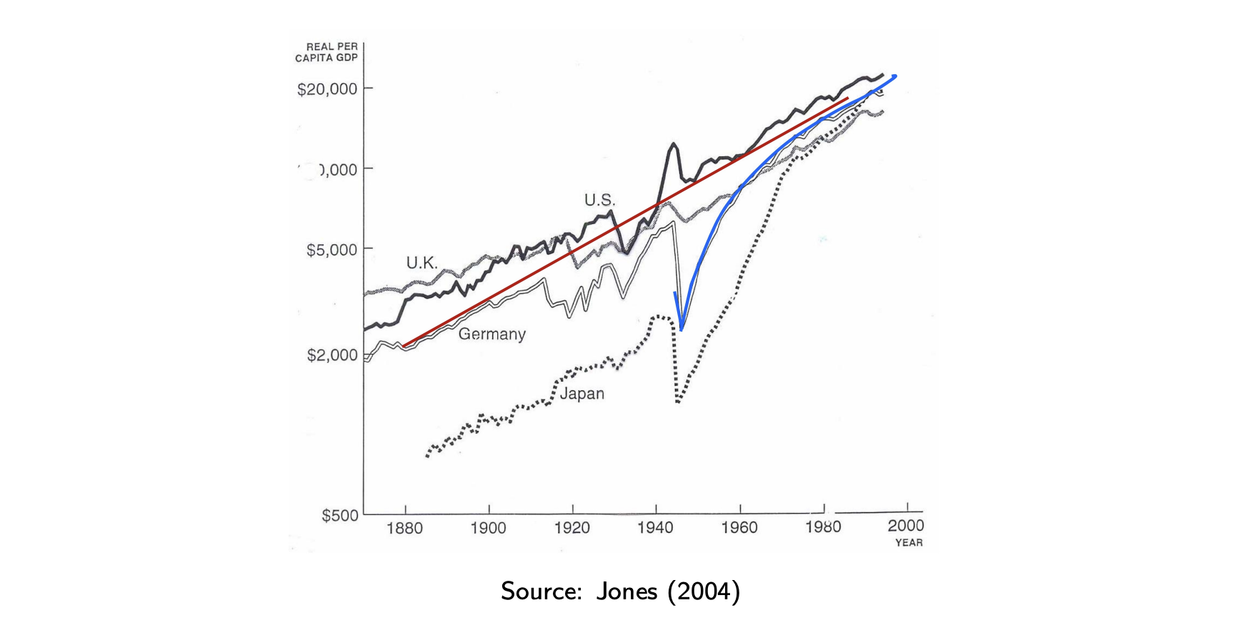
A shock to the capital stock has temporary (but no long-run) effects.
Example: the Second World brought a shock to the capital stock:
We now ask which saving rate maximizes steady-state consumption :
We can then rewrite:
and substitue the steady state condition for capital per effective worker:
so we eliminate and we write consumption as a function of :
that can be maximized by applying the first-order condition:
whose solution is characterized by:
which is called the Golden Rule of Capital Accumulation.
Note that, for the Cobb-Douglas production function, and that an economy with is dynamically inefficient.
Implications of the Solow Model:
- long-run growth per-capita is only driven by technological progress
- in the long-run, capital accumulation is a consequence of growth in technology
- in the short run, growth is faster for countries far away that their steady state.
6. Money holding: Inflation and Monetary Policy
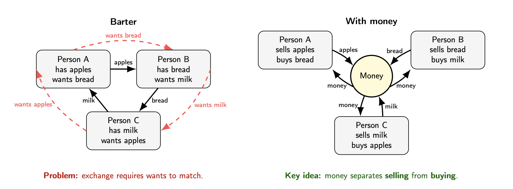
In barter, each side must want exactly what the other side offers. Money solves this by providing a generally accepted medium of exchange.
Fiat money has value because people expect it to be accepted by future exchange. This expectation is self-fulfilling as long as confidence is maintained.
The dollar is the strongest convention man has ever invented
In economics and monetary economics, money is typically defined by its functions:
- unit of account
- medium of exchange
- store of value
A practical definition: money is the set of instruments that are widely accepted at par (at par means: dollar is dollar, no due diligence or questions asked) to settle obligations and make payments.
Note that, according to the economics and monetary definition, Bitcoin (and other cryptocurrencies) are not a form of money: they usually miss the unit-of-measure function and the medium one.
Is bitcoin money? And what that means [Paper]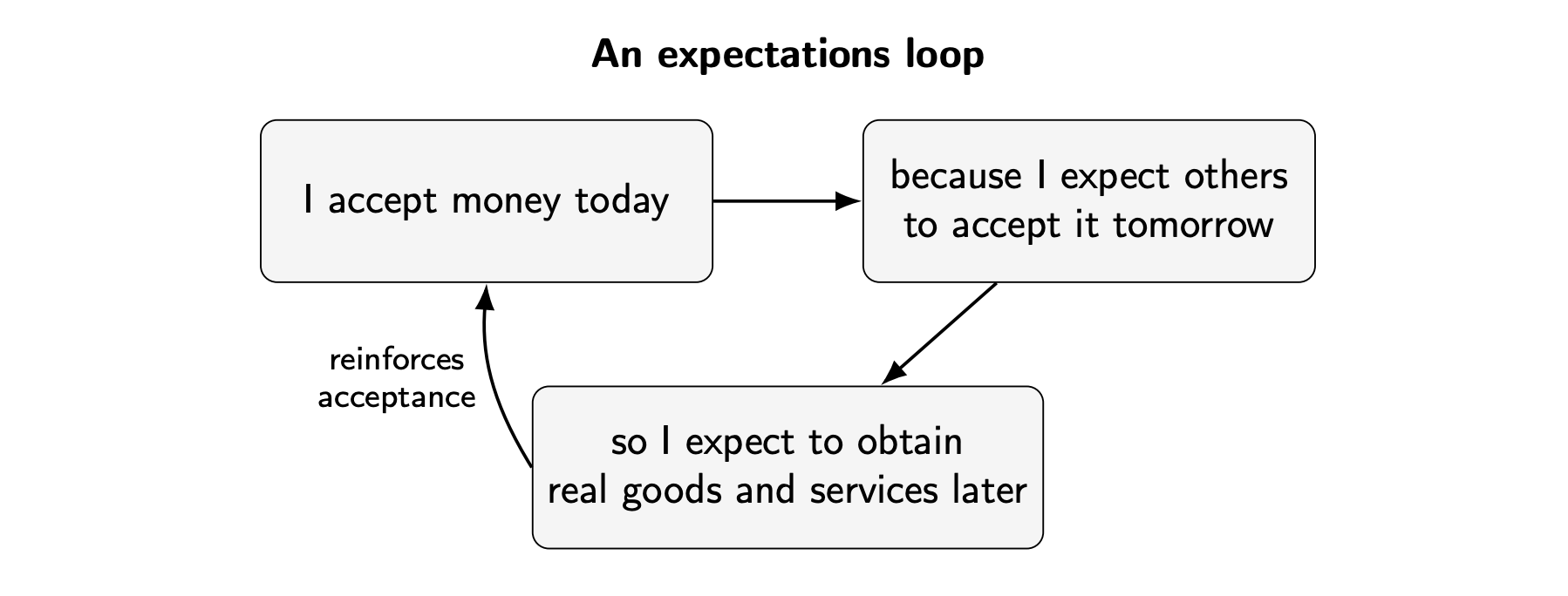
| Instrument | Issuer | Users | Role |
|---|---|---|---|
| Cash | Central bank | Everyone | Public central bank money |
| Reserves | Central bank | Banks | Interbank settlement asset |
| Deposits | Commercial banks | Households, firms | Main money in everyday payments |
In the current economic system, cash doesn't play a major role anymore
- In Switzerland (december 2025): banknotes and coins represented the of aggregate money M1.
The two-tier structure
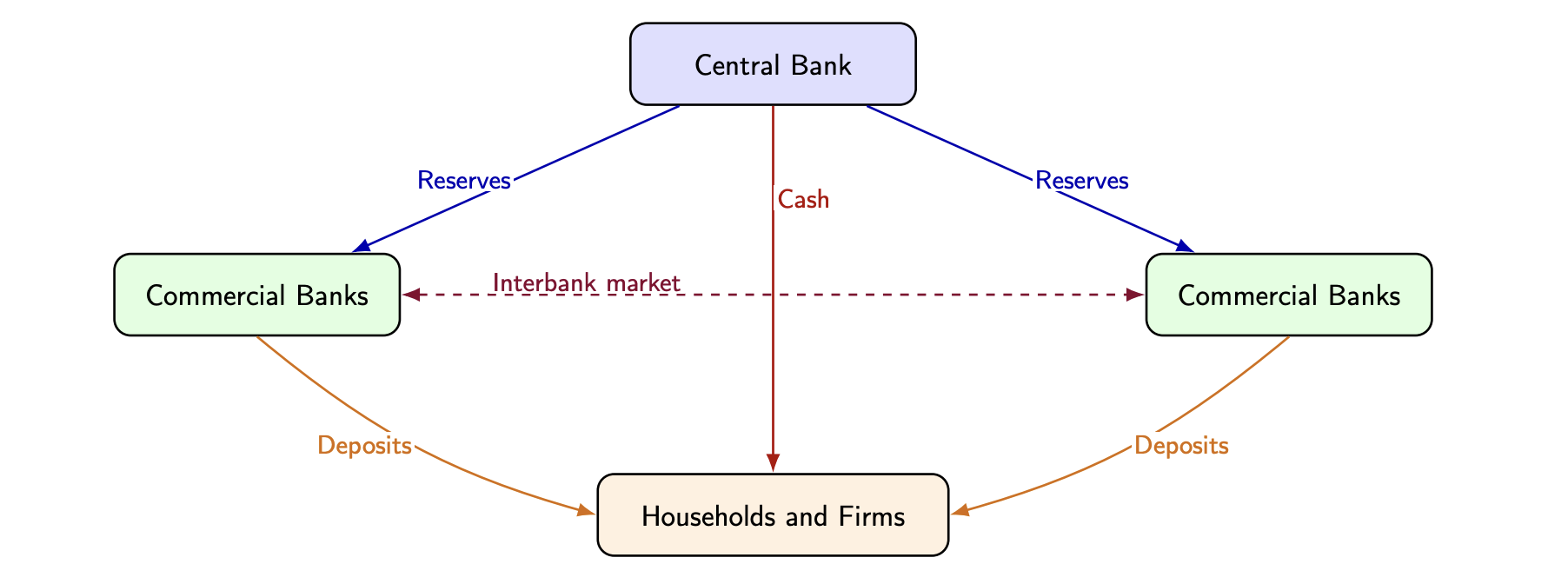
A bank transfer is essentially: a message + a balance sheet update
It can be broken down in two steps:
- Clearing: who owes what to whom?
- Settlement: how are obligations discharged (with what asset)?
In the two-tier system, interbank settlement uses central bank reserves.
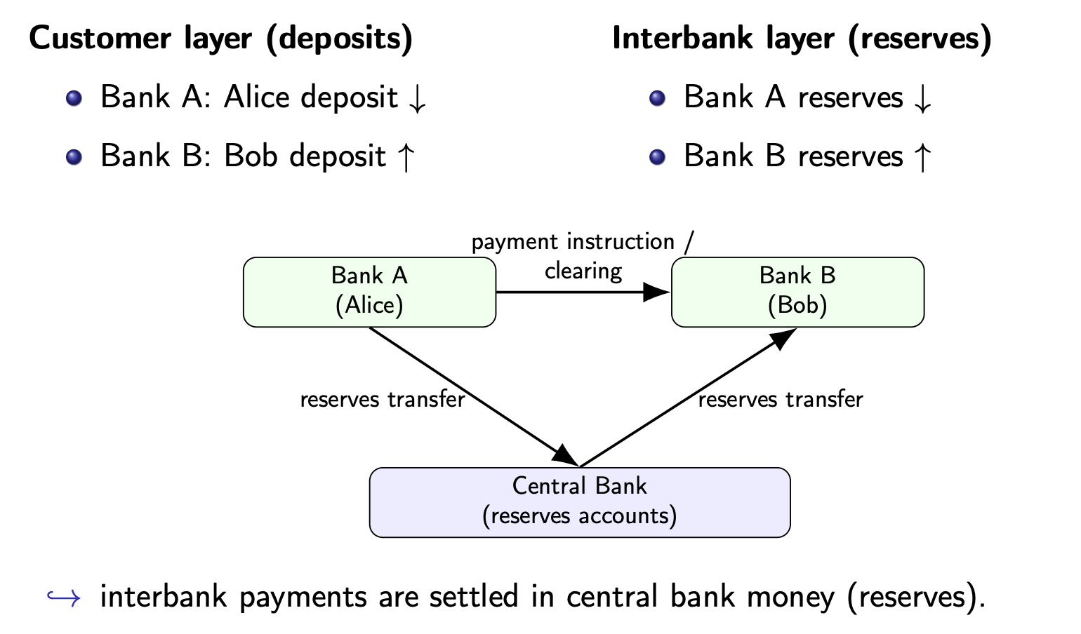
Let's consider the following transaction: Alice transfers to Bob
- Alice instructs Bank A to transfer 10 to Bob.
- Bank A debits Alice’s deposit account by 10.
- Bank A sends the interbank payment instruction into the payment system.
- At the central bank layer, Bank A’s reserve account is debited by 10 and Bank B’s reserve account is credited by 10.
- Bank B credits Bob’s deposit account by 10.
- The payment is complete once the interbank obligation has been settled in central bank money.
- Incoming payments from other banks
- Borrowing from other banks or the central bank (a bank borrows from another in the interbank market, a bank borrows from the central bank through central bank lending operations against collateral).
- Selling assets.
Banks can redistribute reserves among themselves, but only the central bank can create reserves for the system as a whole.
How is money created?
-
Cash (banknotes and coins): cash is a central bank liability issued physically (liability cash is recognized as a claim on the central bank's balance sheet cash is accepted at par by the central bank and the state it functions as "final money" on the economy).
- when a central bank issues cash typically: banknotes (liability) increase and assets (typically something received in exchange) increase.
- When a person withdraws cash, the commercial bank gives away cash and its reserve account at the central bank is debited the central bank's liability (cash) is now held by that person, not the bank anymore cash issuance itself is just a change in who holds the liability.
-
Reserves: they are central bank electronic liabilities. They are created by the central bank when:
- the central bank buys assets from banks. In this cases, the seller's reserve account is credited net reserves in the banking system increase. (note that, unlike a household or a commercial bank, the central bank is the issuer of the monetary unit the creation of money is "just" an accounting entry on its books)
Central bank buys bonds increases banks's reserves and lowers short-term interest rates eases financing can boost spending (demand) if demand supply inflation.
Central bank sells bonds lower reverses tightening liquidity higher short-term rates.
-
Commercial Bank Money (deposits)
- Created electronically, banks expand their balance sheets and credit deposit accounts (main case: banks make loans, some other options include banks buying assets from non-banks).
The Bank balance sheet can be simplified in:
- assets: loans, securities, reserves
- liabilities: deposits, wholesale funding, equity.
Example: a new loan of to a customer increases assets and liabilities by . In this case units of money (deposits) are created.
The bank doesn't need to "find deposits first" to make the loan.
Bank can create deposits ( give loans) and expand their balance sheet, but there're some limits:
- capital and leverage constraints
- liquidity constraints
- profitability and risk: credit risk, funding cost, competition...
- borrower demand
- monetary policy
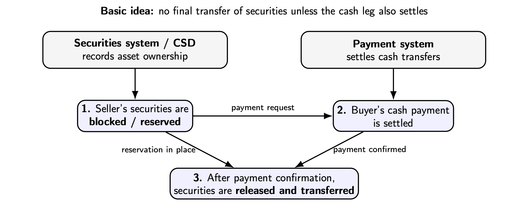
In securities trade, the buyer owes cash and the seller owes securities. If the two legs are exchanged sequentially, one side may deliver while the other side fails. This creates the principal risk problem in securities trade, since there's exposure to the full value of the trade, not just the "replacement" cost.
Delivery versus Payment (DvP) was designed to solve this problem.
Current frictions in payments and settlement:
- cross-border payments can be slow, costly and opaque (multiple intermediaries, different time zones etc...)
- settlement is often fragmented across different ledgers and institutions (example: in DvP cases the cash leg and the asset leg may sit on different systems)
- real-time 24/7 settlement is not universal (many systems are still limited to operating hours)
- programmability is limited (conditional payments, automated settlement and integrated DvP are difficult to implement)
- access to central bank money is restricted (households can old cash, not reserves, for digital settlement, most users rely on commercial bank money)
The current system works very well in many domestic settings, but it is not frictionless, especially across borders.
| Form | Limits as medium of exchange | Limits as store of value |
|---|---|---|
| Cash | not digital; inconvenient for remote or large payments | costly to store in large amounts; theft/loss risk; no interest |
| Deposits | rely on banks and payment systems; not always instant; cross-border frictions | exposed to bank risk above insurance limits |
| Reserves | not available to the public | very safe, but only for banks / eligible institutions |
New forms of money: crypto, stablecoins, tokenized deposits, CBDC
Crypto-asset
Crypto-assets (like Bitcoin) are not typically a claim on an issuer: no underlying liability or redemption at par.
They are native digital assets: transfer and settlement take place on their own ledger and their value is market-determined and often highly volatile.
Generally speaking, they often function more like a speculative asset than as money.
A stablecoin is a digital token designed to maintain a stable value relative to a reference asset (usually a fiat currency).
The biggest ones are currently (March 2026) Tether (USDT) and USDC, both tied one-to-one to the US dollar.
They are typically issued by a private entity and backed by reserve assets, together with a redemption premise. In the past, there were also some algorithm-backed stablecoins (see for example TerraUSD).
Unlike unbacked-crypto assets, stablecoins aim at price stability in the unit of account but, unlike deposits:
- they operate outside the banking framework
- they are tradable on the secondary market
- transfers can settle without interbank settlement in central bank money
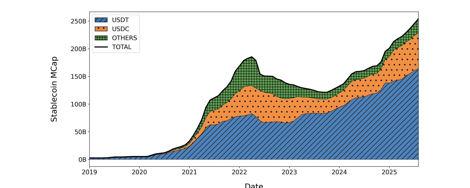
Currently (March 2026) the total stablecoins market is about Bn USD. The two biggest ones USDC and USDT account for more than 90% of the market cap.
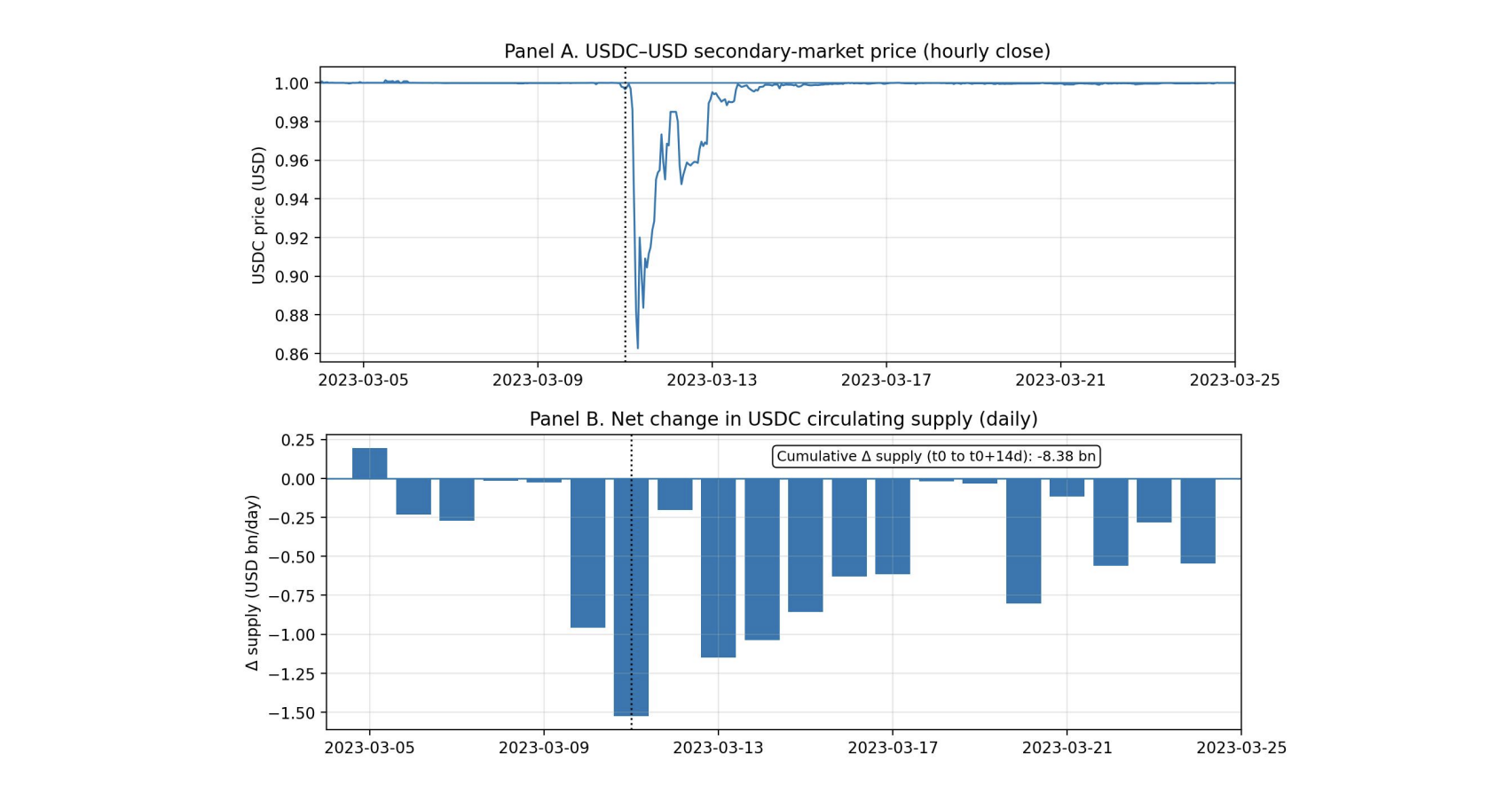
They have been "relatively" stable in the past:
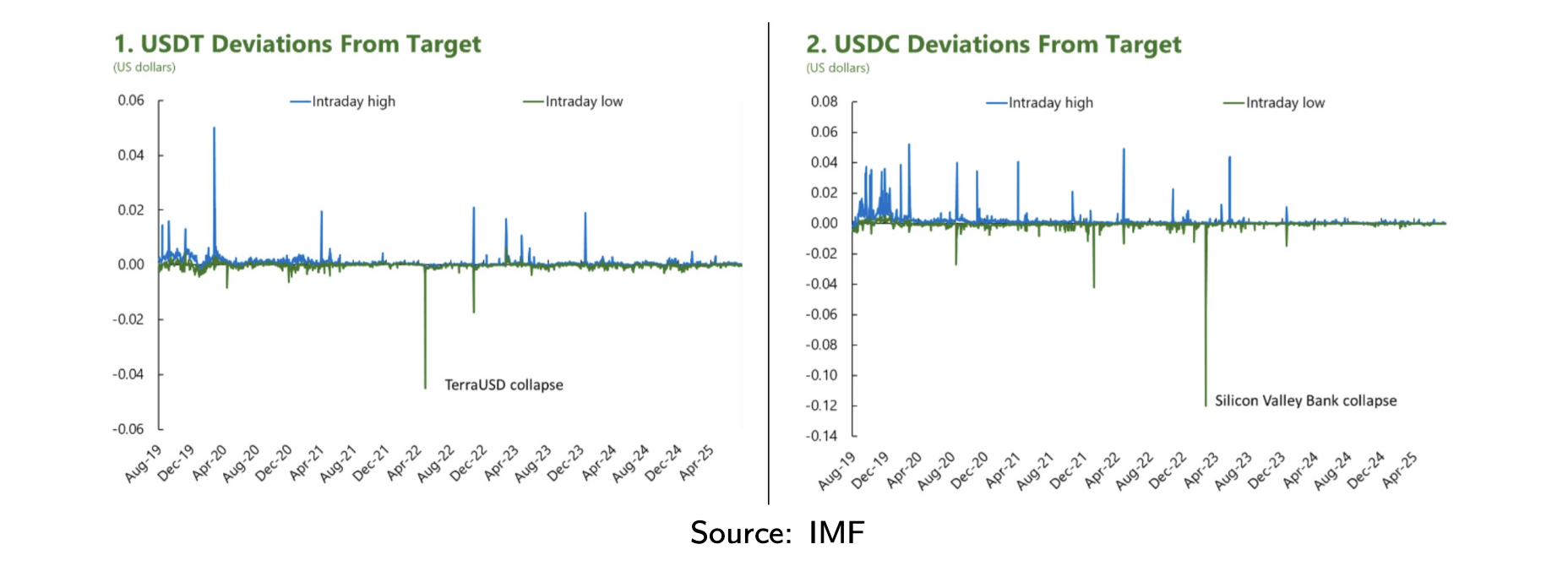
But stress episodes happened. In March 2023, for example, USDC came under stress during the Silicon Valley Bank failure and a portfolio of Circle's reserves (Circle is USDC's issuer) became temporarily uncertain.
What are stablecoins currently used for? (March 2026)
- Within the crypto-markets:
- as a relatively stable trading and settlement asset
- as collateral and liquidity in DeFi (decentralized finance)
- as a place to "park" value between more volatile positions
- Beyond crypto-markets:
- cross-border transfers
- dollar access in some countries
- digital payments on a token-based system
- to bypass restrictions in traditional financial systems (example: capital controls, anti-money laundering (AML) or combating the financing of terrorism (CFT) safeguards)
Still, there are several core risks: reserve quality, redemption/run dynamics, governance and integrity, AML issues and bank disintermediation.
Note that a stablecoin-dominated system would be a distinct monetary architecture from today's one, with privately issued settlement assets potentially operating outside the traditional two-tier system.
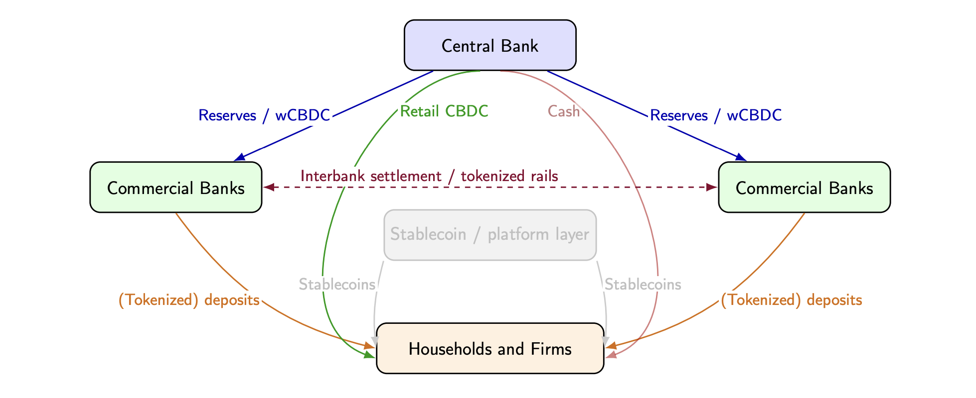
An alternative is CBDC (Central Bank Digital Currency) + tokenized deposits that is mainly a modernization of existing forms of money within the current architecture.
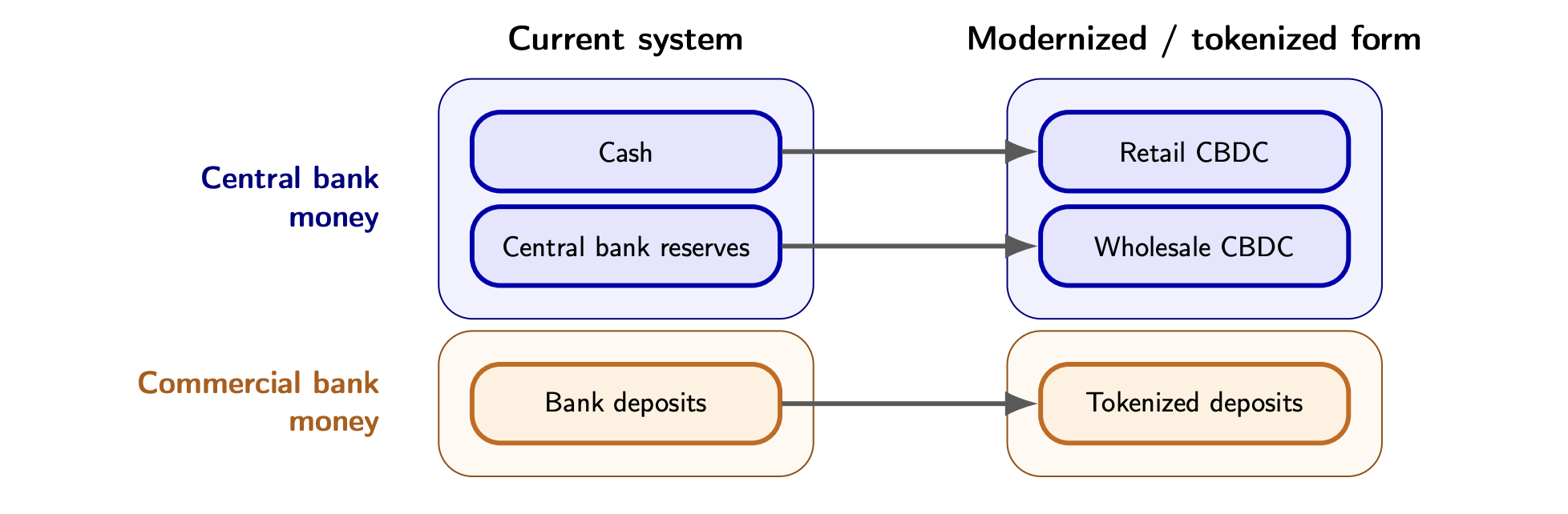
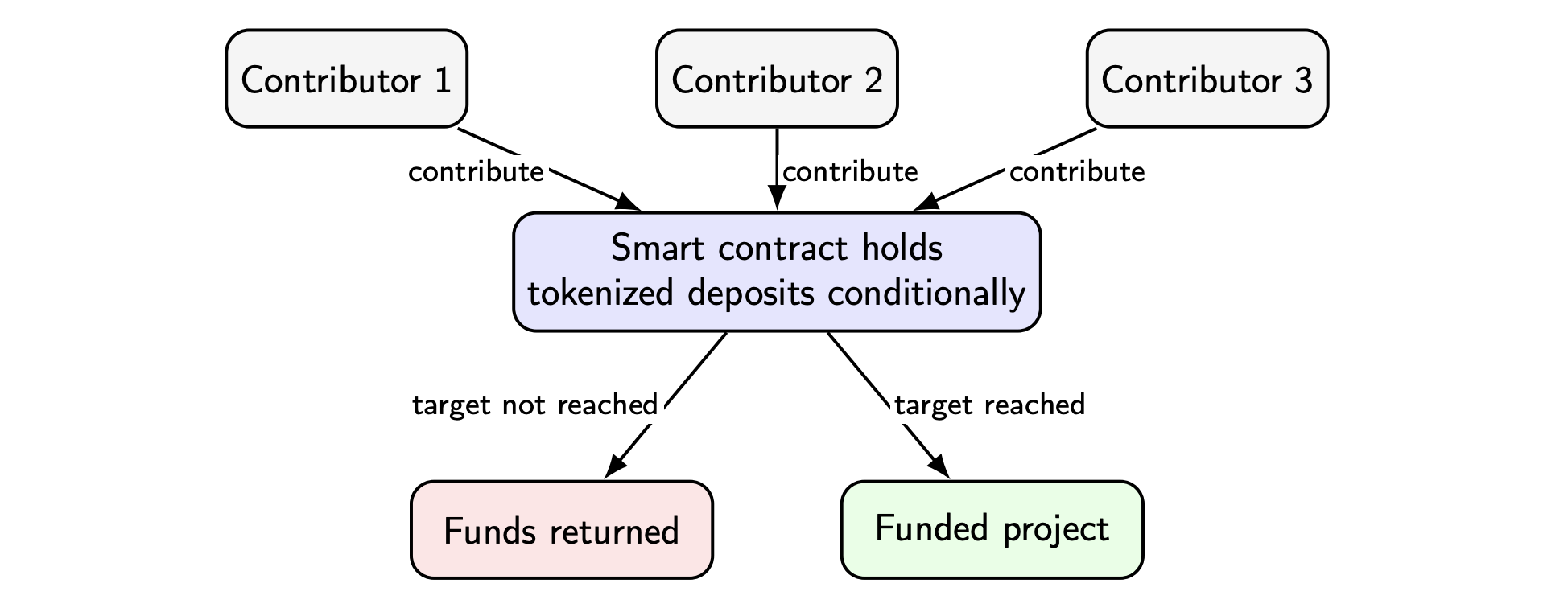
A tokenized deposit is still a bank deposit (a claim on a regulated commercial bank) but it's represented as a digital token on a programmable platform, often using DLT (decentralized ledger technology). It preserves the two-tier monetary system while still changing the transfer and settlement infrastructure, promising greater programmability and potentially more integrated settlement in tokenized markets.
This would be part of a broader trend: not only money, but also bonds and contracts can be brought onto programmable digital rails.
Indeed a token can bundle both information about an asset or claim and the rules governing how it can be used.
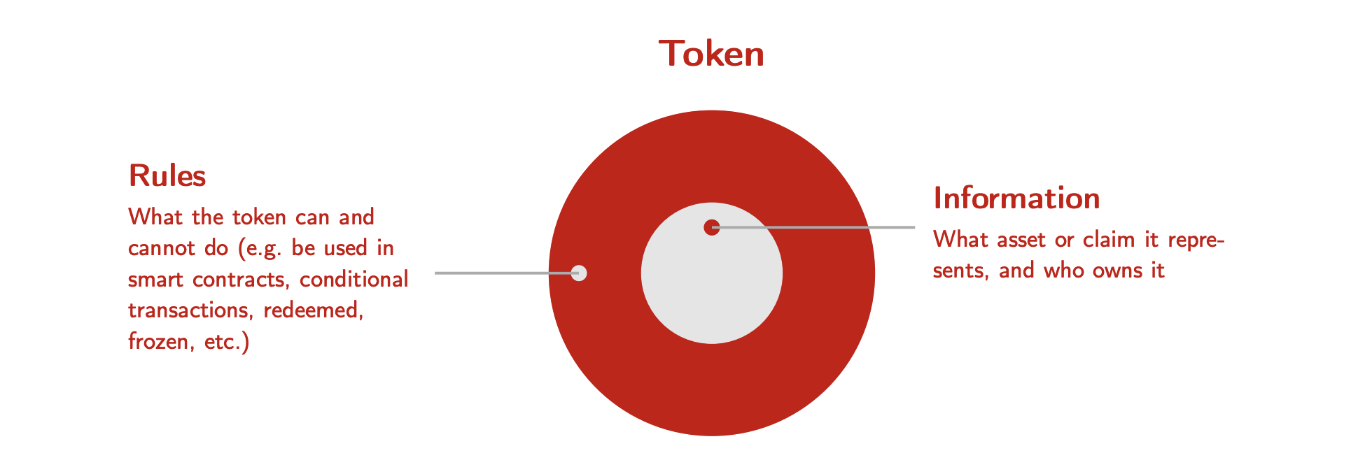
If the target is not reached the funds are automatically returned, reducing the risk of fraud or delay.
wCBDC are Digital Central Bank Money for banks and financial institutions only, they are economically close to the central bank reserves, but potentially with new functionalities enabled by the tokenization.

Retail CBDC are a digital form of central bank money for the general public, often with a token-based design, an intermediate model and more privacy and offline capabilities.
Often described as "digital cash", but its design can differ substantially depending on policy goals and they would be more than a new payment technology (a now monetary architecture choice!).
Currently (april 2026) the world is still not ready for this system:
- advanced pilots in wholesale market infrastructure for wCBDC are ongoing
- The SNB Project Helvetia on SDX and the Eurosystem DLT work
- In China, large-scale pilots (e-CNY) for rCBDC are in place
- The US is still hostile to rCBDC.
7. IS-LM Model and Open Economy
The monetary policy goals can be summarized, as in the standard US textbook by Frederic Mishkin, in:
- low unemployment (high GDP)
- economic growth
- price stability
- interest rate stability
- financial market stability
The problem is that this multitude of goals often cannot be reached simultaneously, requiring some trade-offs.
We speak by of discretionary policy the central bank can choose its policy period by period.
We speak of rule-based monetary policy policy is constrained by a previously announced rule or commitment.
At first look, a discretionary policy seems superior to a less-flexible rule based, however, current policy affects private expectations for the future, discretion may lead to inferior outcomes.
(Since the early 1990s, many countries have moved towards a more rule-based monetary system, largely independent by the government).
On the other side, discretionary policy has some major drawbacks, and the most important is the so-called Time Inconsistency Problem.
The Time Inconsistency Problem
The classic analysis of these problems comes from Kydland and Prescott, that, for this achievement, received the Nobel Prize.
A plan is time inconsistent if it is judged optimal at , but at the same decision maker prefers to revise the plan, even though no new relevant information is available and the current environment has not yet changed.
(This problem is also linked with credibility: announcements are no longer credible if one knows that they will later changed).
The TI Problem in Monetary PolicyA central bank knows that it cannot influence real variables in the long run but it can influence the inflation rate; it will ex-ante formulate its policy in such a way that it results in an optimal inflation.
However, if the central bank can influence real-variables in the short run, it will be tempted to deviate from the previous policy.
Therefore, it is no longer time-consistent.
The equilibrium is thus an inflation rate which is higher than socially desired, but without changing output in the long run.
(The solution would be a independent CB with rule-based monetary policy).
The Barro-Gordon (1983) Model I
The model describes a CB that bases its actions on a social welfare function (discretionary monetary policy).
The CB can directly choose an inflation rate for the short-run.
The private sector is the second player and it is described by rational expectations, we then model a strategic game with simultaneous decisions.
The social welfare function can be defined as:
or as a loss function as:
with:
- : constant
- : inflation rate
- : output
- : target inflation (we assume here )
- : target production.
The Phillips curve summarizes the interplay between real and nominal variables:
with:
- : natural output ( with )
- : constant
- : expected inflation
Intuition: The only way the CB can trick output into rising above its natural level () is by creating "surprise inflation" ().
The private sector has rational expectations, that is:
This immediately implies that (via the Phillips Curve) in equilibrium must satisfy:
Unfortunately, with discrete-monetary policy, this is not what we get in equilibrium!
So let's go back to the loss function and let's substitute the Phillips curve:
We now minimize this function with respect to :
that leads to the Monetary policy reaction function:
Together with the reaction function (expectations) of the private sector, , the equilibrium is:
The equilibrium output is then: .
So the discretionary equilibrium delivers positive inflation but no increase in real output. That is the classic inflation bias: the policy maker would like to raise output above the natural level, but rational expectations eliminate the real gain.
In this toy model, the commitment benchmark is and .
Let's now suppose that (the expected inflation) is exogenous. The loss function in this case is:
If we substitute the Phillips Curve and we calculate the first derivative w.r.t :
that leads to:
if it holds that :
Intuition: the central bank sets the inflation a bit higher than its target to bring y closer to .
We immediately notice that the first solution, , is time-inconsistent.
Indeed, if , there's nop surprise inflation and the output would stays at its natural level , still achieving the inflation target .
However, this plan is only "ex-ante" optimal and in reality ("ex-post") will break since the CB has an incentive to cheat one expectations are done.
Indeed, if the private sector actually believes the CB can set low inflation , the CB could just cause the a tiny bit of surprise inflation to boost output .
For this reason, the announcement is not credible. Furthermore, in a world of rational expectations, people understand in advance the CB's incentives and anticipate this behavior.
For these reasons, since discretionary policy does not provide the desired results, it is socially-optimal to delegate monetary policy to an independent institution, that then credibly announces .
Along these lines, the constitution of the ECB was drafted.
Possible extensions of the Barro-Gordon Model:
- Look at repeated games instead of a one-shot game
- Include information imperfections
- Take supply-shocks into account
- Model wage settings
also with these changes, the results presented here remain qualitatively very robust.
8. Bank Runs: The Diamond-Dybvig Model
Banks hold only a fraction of their deposits as cash and reserves. The remainder of banks' assets is illiquid. this makes banks prone to bank runs
A bank run is often characterized by a sequence of events:
- depositors lose trust in a bank's viability
- depositors withdraw demand deposits
- the bank must liquidate its long-term assets to serve its short-term liabilities
- the bank defaults if the assets' liquidation value is too small for the bank to serve all withdrawals
a "not so healty" bank can fail due to a bank run:
- a bank runs out of liquidity due to an unexpected liquidity shock
- yet, the market value of its (illiquid) assets exceeds its liabilities
- the bank defaults if it must fire-sell its assets at low prices.
Note the distinction between:
- solvency risk: long-term risk on the balance sheet, given by excessive debt, declining asset values
- liquidity risk: short-term risk on the cash flow (availability of liquid assets) caused by a poor cash and timing manageent
Therefore:
- A company (bank) can be solvent but not liquid (if it has enough assets but lacks the cash to meet immediate obligations).
- A company (bank) can be liquid but not solvent (if it has enough cash to meet short-term obligations but not enough assets compared to long-term liabilities)
The Diamond-Dybvig Model
This model formalizes bank runs in with two important features:
- banks offer deposit contracts, which provide risk sharing and liquidity insurance in case of shocks on consumption needs
- deposit contracts can have undesirable bank run equilibria in which all depositors panic and withdraw immediately, including the ones who would prefer to consume late.
The Consumer's perspective
We start with a slightly simplified version of the environment.
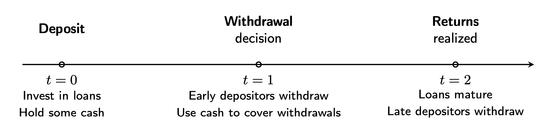
- there are three dates,
- there is a mass of ex-ante identical, risk-averse agents
- there are two types of investment technologies:
- storage yields at
- long-term investment yields at but only it it must be liquidated early at (fire sale) early liquidation is costly!
At , all agents are identical. They don't know in advance when they will need to consume.
At , each agent learns their type (which is a private information):
- with probability they will need liquidity early ()
- with probability they can wait and consume later ()
(we can interpret as the probability to be hit by a liquidity shock)
Suppose now that one unit of the good is available at you at . There are two ways to use it:
- storage (liquid asset)
- long-term investment offering a return while being illiquid
Suppose that each person acts alone, without a bank. Then each individual must deal with the possibility of needing early consumption by itself, creating a difficult choice: keep in storage and be liquid or invest for the long-term and risk an early-liquidation loss.
Without a bank, each person bears their own liquidity risk.
Optimal allocation for an individual depends on and his degree of risk-aversion.
Pooling helps because, even if each individual is uncertain about their own liquidity needs, in a large group, the fraction of people who need early consumption is often fairly predictable by the Law of Large Numbers, a fraction will need liquidity early at .
Economic intuition (Liquidity Insurance): if many people pool their funds, some can withdraw early, while the rest of the resources can remain invested long term.
The Bank's perspectiveBanks collect deposits from many households. They can then invest a share of these funds in long-term assets and keep a share as liquid.
- all depositors are then offered the possibility of withdrawing on demand
- they participate in the returns of the asset portfolios held by banks through interest earned on their deposits
- Banks perform maturity transformation:
- they hold relatively illiquid-long-term assets
- they issue relatively liquid-short-term liabilities
(This mechanism allows society to invest in productive long-term assets while agents with unexpected early consumption needs can still access funds at any )
As a consequence:
- more resources can remain invested in high-return long-term projects.
- depositors participate in these returns with interest on deposits
- early consumers gain access to liquidity they need it
But, at the same time, this structure also creates fragility: if too many depositors demand liquidity at once, the bank can run into trouble.
In particular, this mechanism becomes fragile if a larger fraction tries to withdraw early since a bank can promise liquidity to each depositor individually, but not to all depositors simultaneously (the bank is liquid only against "normal" withdrawal demand, not against everyone withdrawing at once)
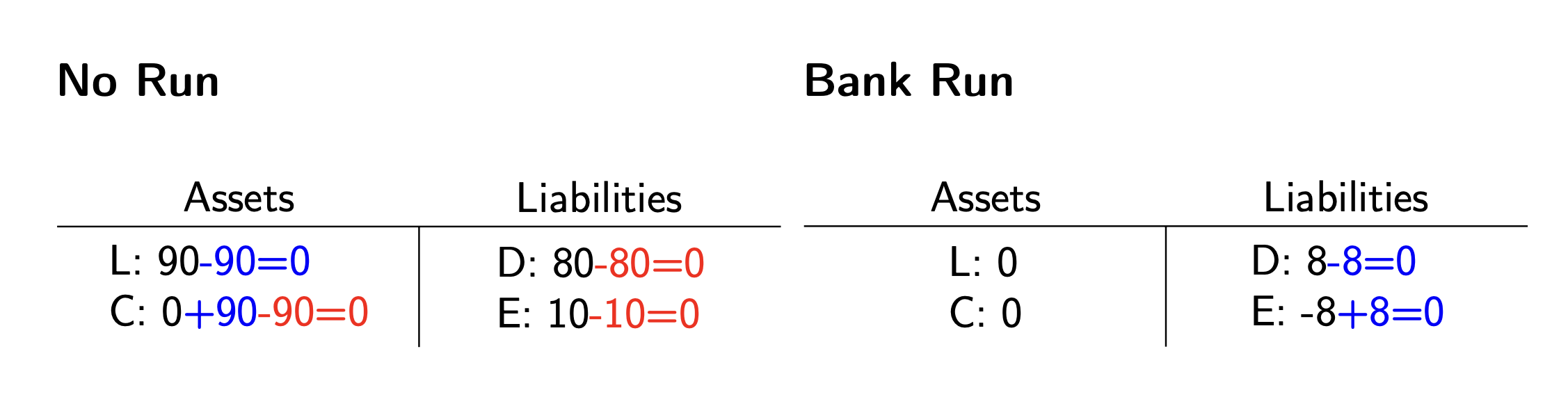
Assume now the following:
- loans repaid at
- loans can be sold off at but at a fire-sale discount of 20%
- there are 20 depositors of the early type, 80 of the late type and 10 equity holders owning the bank
- each agent owns 1 unit of funds in
- for simplicity: no interest is paid on loans or deposits, eliminating the need to account of interest income or expense
At , if we consider Loans (L), Cash (C), Deposits (D) and Equity (E):
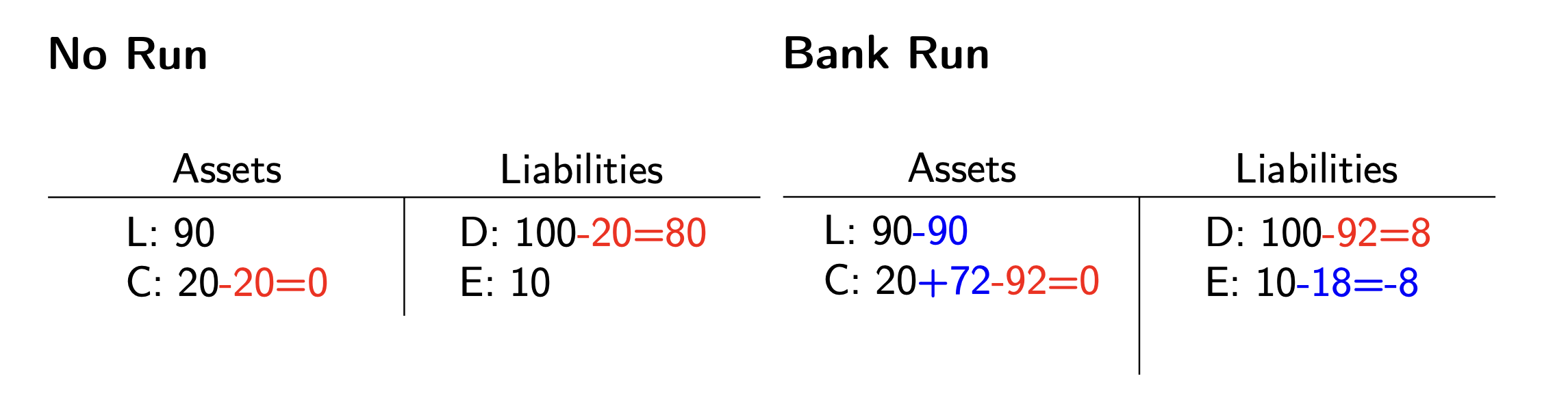
At there's limited liability: shareholders cannot be forced to recapitalize, so the remaining 8 units of deposits are written off; they get nothing.
In general, if only people with real liquidity needs withdraw at the bank can still meet these withdrawals from:
- its liquid reserves
- if needed; limited liquidation of long-term assets in this case, the remainin gassets can stay invested and generate return at .
The panic-scenario
Now suppose that many depositors try to withdraw at , including those who could actually wait. In this case, the bank must liquidate a large amount of its long-term assets early (remember that early liquidation is costly), so panic destroys value.
if too many depositors demand liquidity at once, the bank may be forced to sell long-term assets at a loss and may be unable to satisfy everyone in full.
For a depositor who does not need funds early:
- if they expect the others to remain calm/rationale, it is best to wait until
- if they expect many others to run, waiting becomes dangerous:
- the bank may run out of liquidity
- long-term assets may be liquidated at a loss
- late withdrawers may receive less/zero
The first-mover advantage
Banks typically serve withdrawal requests in the order in which they arrive
those who arrive early are more likely to be paid in full
In a panic, it can be individually rational to withdraw early simply because others may do so first
this first-mover advantage is the central ingredient of the Diamond-Dybvig logic.
If everyone expects a run, then running becomes individually rational and so the run occurs.
Liquidity Crisis vs Solvency Crisis
A bank can fail even if it is solvent the problem may be of liquidity, not necessarily of solvency
- if the assets could be held to maturity, they might be sufficient to cover the bank's obligations
- if the bank is forced to liquidate them early under stress, it may realize losses and fail
In general, a liquidity crisis arises because fund are needed now, a solvency crisis arises because assets are worth too little
The Diamond-Dybvig model is a story about a liquidity crisis that can turn into a solvency crisis
Note that crisis can also begin in the opposite direction: doubts about solvency can trigger a liquidity crisis.
From classic bank runs to modern digital banks
In this model, depositors try to withdraw cash at the same time. However, in modern banking systems, this often no longer means queuing up physically at the bank. Instead, the run can be even more frictionless and consist in:
- rapid digital transfers to other banks
- shift into money market funds or Treasury Bills
A modern bank run is often not a run into cash, but a run out of a bank's liabilities and into alternative stores of value.
Policy, interpretation and limitsThe previous model doesn't state that banks are undesirable, banks are indeed socially useful because they provide liquidity insurance. The policy is therefore not to eliminate banking, but the challenge is to preserve the good equilibrium while ruling out the run equilibrium.
Crises solutionsOne classic solution is a suspension of convertibilitiy if cash reserves are depleted in , this prevents runs:
- the bank stops withdrawals in after first 20 depositors in queue withdrew it closes down initial cash reserves are depleted
- this ensures that loans can mature without fire-sales.
In this case, this action restores confidence:
- late types know they are safe and there is no reason to withdraw early
- early types can each withdraw successfully at because late types have no incentive to run
But this not necessarily work well if is unknown or understimated.
Another solution is deposit insurance:
- if depositors know their funds are protected even if the bank comes under pressure, then the incentive to run is reduced
- in this case patient depositors no longer need to rush to withdraw early
A further solution is a Lender of Last Resort:
- the central bank can provide liquidity to a fundamentally healthy but illiquid bank
- this prevents inefficient fire-sales and disorders that can lead to failure
but these solutions can raise other issues, such as moral hazard:
- depositors may pay less attention to bank risks
- banks may have stronger incentives to take risk
its downside risks are partly absorbed by the public sector, private actors may take on more risk than is socially desirable.
This is why modern banking systems do not rely on deposit insurance or LOLR, they also provide a prudential framework to limit risk-taking in the first place. Two core elements are:
- capital regulation: banks must have enough loss-absorbing equity
- liquidity regulation: banks must hold enough liquid assets
a stable system requires both crisis-management tools and ex-ante regulation.
Note that whether a bank can obtain emergency liquidity from the central bank depends on whether it is illiquid or insolvent:
- panic runs reflect temporary illiquidity (LOLR can bridge the gap and prevent fire sales);
- fundamental runs reflect true insolvency (LOLR cannot restore solvency and recapitalization/fiscal measures are required).
9. Crises in Market Economies
Crises can be either single (as standalone events: financial market, real estate, currency, public debt, banking, private debt etc...) or the combination of two or more aspects at the same time.
2008 Banking CrisisFor example, during the banking crisis in 2008, house prices in the US dropped by about 20-30% many households suddenly saw the value of their houses fall below the amount they still owed to the bank (this is called negative equity) they could no longer refinance their mortgage or sell the house to repay the loan many borrowers became stressed or defaulted private debt crisis.
In simple terms: the value of the house falls a lot, but the debt stays the same, the borrower is trapped. If many households face this situation at the same time, the problem spreads from the housing market to the whole economy.
Banks, in particular, had losses on Mortgages Backed Securities (MBS) private borrowers defaulted.
A MBS is a security backed by mortgages, it represents an interest in a pool of mortgage loans).
Unlike a bond, in the MBS case the cash flows are not fixed, they depend on mortgage repayments, prepayments (borrowers can refinance or pay early), higher default risk and the discount rate used by the market.
For many agency MBS, people often use an option-adjusted spread approach (extra yield added to a benchmark so the bond's model price matches the market price accounting for embedded options), which means that the bond is priced as the present value of the cash flows after adjusting for the prepayment.
Banks had very little equity (in the extreme case: UBS and some other around 2% of total assets) so:
- some banks could not absorb losses and started to move toward default
- healthy banks were affected through interbank loans
many more banks moved to default danger of banking system collapse.
Since a collapse of the banking system would have cause large losses (in GDP, employment, panic etc...), the government rescued banks.
As a consequence, in some countries public debt increases so much that a public debt crisis occurred.
What could have been done to prevent such a crisis?
- increase equity ratios in banks so they can absorb losses (banking crisis)
- reduce public debt over time (public debt crisis)
- require at least 20% of house value as equity investment (private debt crisis)
The criteria to choose a good instrument usually are:
- is the criteria effective?
- does it have negative consequences for the economu today or in the future?
- does it burden taxpayers excessively?
From a crisis-management point of view, the goal is simple:
- stop panic in the short run
- avoid a collapse of credit to households and firms
- stabilize output and employment.
The main actors and tools are:
-
Central Bank (liquidity manager)
- provides emergency liquidity to banks (typically short-term loans against collateral)
- lowers policy rates to reduce funding stress
- can expand its balance sheet to calm markets.
-
Government / Treasury (solvency backstop)
- recapitalizes weak banks (injecting public capital and becoming shareholder if needed)
- supports restructuring or temporary public control of failing institutions
- can purchase or ring-fence distressed assets to reduce uncertainty
- can provide targeted fiscal support to households and firms.
-
Public Guarantees (confidence tools)
- stronger deposit guarantees to prevent retail bank runs
- guarantees on interbank funding to restart lending between banks
- guarantees on loans to firms to avoid a credit freeze in the real economy.
-
Standard macro policies (demand stabilization)
- monetary easing: lower short-term interest rates
- fiscal expansion: higher government spending and, in some cases, temporary tax relief.
-
Direct government/CB interventions:
- providing loans to firms by the government
- buying up toxic assets by the central bank in the market.
Intuition: the central bank mainly addresses liquidity, while the government addresses solvency and supports demand. Using both together is often necessary in systemic crises.
Main trade-off: stronger support reduces the probability of collapse today, but can increase public debt and moral hazard tomorrow.
In 2008, new funds should have been injected, deposit guarantees increased, interbank loans provided, and the short-term interest rate lowered.
Note that measures 4 and 5, at least alone, do not resolve a banking crisis!.
Public Debt Crisis
The most common reasons for a public debt crisis are:
- Persistent deficits over many years: governments spend more than they collect in taxes, not only in recessions but often also in normal times.
- Large extraordinary shocks: wars, natural disasters, banking rescues, and major infrastructure programs can suddenly raise debt.
- Higher interest costs: if interest rates rise while debt is already high, debt dynamics can deteriorate quickly.
In theory, a Keynesian approach suggests: deficits in recessions, surpluses in expansions. In practice, many governments do the first part, but not the second one.
The common pool problem means that many political actors push for spending that benefits their own group, while the tax cost is spread across all taxpayers and often shifted to the future. As a result, total spending can become too high.
Typical political mechanisms behind debt accumulation are:
- Political budget cycles: before elections, policymakers may increase spending or cut taxes to gain support.
- Delayed stabilization: even adjustment is needed, political conflict can postpone decisions, so debt keeps rising.
- Fiscal illusion: voters may see the immediate benefit of spending, but underestimate the future cost of taxes and debt service.
The outcome is often asymmetric policy: debt rises in bad times, but is not reduced enough in good times.
To address this, countries use different fiscal rules:
- Balanced-budget rules: budgets should be close to balance over the cycle.
- Debt brakes: if debt rises too much, automatic correction is triggered in later years.
- Stabilization reserves: governments save in good times, then use those buffers in recessions.
- Expenditure rules: spending growth is capped to avoid permanent expansion of public spending.
- Institutional accountability: stronger monitoring, fiscal councils, and political penalties for repeated violations.
Deep dive: Maastricht criteria (EU)
The Maastricht framework introduced two famous reference values:
- annual public deficit should not exceed 3% of GDP
- public debt should not exceed 60% of GDP, or should move clearly toward that level over time.
The economic intuition is simple:
- the 3% limit tries to avoid persistent large yearly deficits
- the 60% limit tries to keep total debt at a sustainable level.
Over time, this framework evolved through the Stability and Growth Pact:
- a preventive arm: countries should keep their structural budget close to a medium-term objective
- a corrective arm: if deficit/debt limits are breached, an excessive deficit procedure can be opened.
In practice, there are also escape clauses for severe recessions or extraordinary shocks (for example systemic crises), because strict consolidation during a deep downturn can worsen the recession.
Main strengths:
- creates common criteria for fiscal discipline
- improves comparability across countries
- reduces the risk that one country's fiscal instability influence others.
Main weaknesses:
- one rule cannot fit all countries all the times
- enforcement can become political and uneven
- complex rules are harder for voters to monitor.
So there is a clear trade-off:
- very rigid rules increase discipline, but can be too harsh in crises
- very flexible rules help stabilization, but may fail to stop debt accumulation.
So the main policy challenge is to combine both credible long-run debt reduction with enough short-run flexibility in major shocks.
A new approach to limit public debt accumulation is a debt-sensitive majority rule:
- the majority needed to approve the budget is 50% if there is no deficit, but the required majority increases as the planned deficit increases.
for instance, a deficit of 1% of GDP may require 55% of votes, while a deficit of 2% may require 60%, and so on.
According to this rule: the higher the planned public debt, the higher the parliamentary majority needed to approve it.
10. Macroeconomic Forecasting
Macroeconomic forecasting refers to the process of predicting future realizations of economic aggregates (GDP, indlation, unemployment, interest rate etc...).
- Forecasting: the process of looking ahead using historical data to predict values at a specific points in the future.
- Idea: Predict where (horizon), given all information available up to to .
- Nowcasting: the prediction of the present, the very near future, or even the very recent past where is very small.
- Backcasting: can have separate meanings:
- Estimating missing data from the past before your data collection began.
- Imagining a specific future and working backward to determine what needs to happen to make it happen.
Several approchaes possible to forecasting:
- judgmental/expert forecasting, based on opinions, intuition, visual data inspection and prior economic theory.
- strengths: flexiblility to incorporate current events of breaks, useful data is limited or unreliable
- weaknesses: subjective to bias, hard to replicate
- time-series model
- machine learning models that learns complex, often non linear patterns from data with minimal prior structur.
- main difference from time-series: ML mainly focused on large unstructured data, it emphazises flexbible and data drive prediction, while TS models rely on explicit statistical structure and assumptions.
- structursal macroeconomic models
- dynamic stochastic general equilibrium (DSGE) models: they model the behavior and the interdependencies between agents based on micro-economic theory they provide a set of equations describing how the economy works.
- Structural model an be either calibrated or estimated (based on macro-economic time-series data)
Time-series Basics
A time series is a sequence . We define the forecast horizon as and we forecast:
to obtain a forecast series:
We define the forecast error as:
The Loss Function defines the criterium for forecast accuracy. Some common examples are:
- Root mean squared forecast error (RMSFE):
- Mean absolute forecast error (MAFE):
The Random Walk forecast model
We consider the simple case in which we want to forecast at period (one-step ahead).
The random walk model is simply:
Conditioning on the information set at time and using :
So the one-step forecast is:
The corresponding forecast error is:
For horizon :
Intuition: the best prediction is the latest observed value, while uncertainty increases linearly with the horizon.
AR(1) forecast model
The autoregressive model of order 1 can be defined as:
where is the autoregressive parameter.
The one-step-ahead conditional expectation is:
In practice, replacing with its estimate , we get:
For steps ahead:
and the forecast error can be written as:
If (stationary case), then as .
Intuition:
- if , dynamics are highly persistent and close to a random walk.
- if , shocks fade out gradually (mean reversion).
- if , the process tends to alternate signs around its mean.
More detail on AR models can be found here!.
Dynamic factor model (DFM) framework
Let the variation in the data be captured by high-frequency factors.
We consider the measurement equation for the dynamic factors :
and the state equation for the dynamic factors:
Firstly, we forecast the factors using the state equation:
Then, we use the measurement equation to forecast observables: