The following notes come from the course Economic Dynamics and Complexity, held by Luca Verginer at ETH Zurich.
For a more practical approach, please refer to the GitHub Reporisoty of the course .
Index
- 1.1 Cobweb Dynamics: a simple model for supply and demand
- 1.2 Basics of Epidemic Models
- 1.3 Supply Chains as Rooted Trees
- 2.1 Growth Models: exponential and logistic
- 2.2 Fishing/Harvesting Model
- 2.3 Growth Models: supply and demand determine price
- 3.1 Common Source Diffusion
- 3.2 Bass Diffusion
- 3.3 SIRS Models
- 3.4 Complex Contagions on a graph: a formal setup
- 4.1 Coupled Dynamics: Lotka-Volterra Predator-Prey Model
- 4.2 Coupled Dynamics: Goodwin's Model (1967), Cycles in Employment and Wages
- 5.1 Discrete Dynamics: Cobweb Plot
- 5.2 Discrete Dynamics: Saturated (Logistic) Growth
- 6.1 Endogenous Cycles
- 6.2 Endogenous Cycles: Kaldor Model (Business Cycle)
- 7.1 Introduction to Networks
- 8.1 Diffusion on Networks
- 9.1 Community Detection: Dirichlet Energy, Rayleigh Quotient and Network Bisection
- 9.2 Network Eigenvector Centralities
- 9.3 Katz and PageRank Centralities
- 10.1 Strategic Network Formation
- 10.2 The Connections Model (1996)
- 10.3 The Co-Author Model
- 11.1 Dynamics of Strategic Network Formation
- 11.2 Spatial Connections Model
1.1 Cobweb Dynamics: a simple model for supply and demand
Consider Supply , Demand coupled via the price with linear dependence.
- Demand responds to price immediately
- Supply responds with lag (production takes time).
The system can converge, oscillate or diverge depending on how supply and demand are sensitive to price.
1.2 Basics of Epidemic Models
A simple Susceptible-infected (SI) model states:
where denotes the inftected contacts per time unit, the infected, the susceptible (healty) individuals. Note that, at the final state everyone is infected.
Assuming that the population is closed and that recovery is not possible, the share of the population infected increases following a logistic growth:
In the early phase: (almost a exponential growth), in the long run .
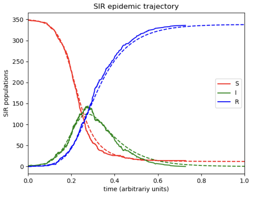
On the other hand, Susceptible-infected-Removed (SIR) model introduces the possibility of recovery, represented by .
The infected people are a transient state and at the equilibrium (the final stage) the disease cannot spread anymore.
In discrete time, the previous expressions become:
1.3 Supply Chains as Rooted Trees
We can represent a chain as a graph , with representing the set of verttices (notes) and the set of edges, that can be directed or not: .
Edges can be weighted () and represent capacity, volume, lead time or reliability of a single link of the supply chain.
We denote by , the degrees (number of connections) of a node has in input (suppliers) and output (customers). A directed tree models an isolated supply chain with source suppliers and root assembler.
In reality, firms have multiple interconnected suppliers and customers, leading to a supply network
Dynamics of networks: how links form:- Networks evolve: entry, exit, mergers, rewiring.
- The simple mathematical rule behind is: (the probability that a node connects to a new node is proportional to its number of degrees)
- The outcome is a heavily-tailed degree with a few hubs and many small degrees.
Dynamics of networks: how goods flow | Continuous Flow (deterministic)
Let's denote by the inventory at node .
The flow balance is given by:
Where is the inflow from suppliers, the outflow to customers or other nodes, the production and the demand.
In matrix form: .
Dynamics of networks: how goods flow | Markov Routing (stochastic)We consider a transition matrix with entries and we denote by the probability of good at each node.
We then have the following dynamics:
2.1 Growth Models: exponential and logistic
We initially study a simple growth dynamic: the compounding interest.
We consider a initial deposit and a nominal annual rate , with interest credited every .
with , we then obtain: .
As , we can switch to continuous time:
The analytical solution of this simple ODE is obtained via separation of variables:
and then, solving for x:
If we instead want to solve the initial value problem with a numerical approximation (Euler's method) we choose a step size and set up a time grid.
At each step, we obtain the gradient at the current point and take a step in that direction. This leads to the Euler update rule:
In python, for example:
def euler(f, x0, t0, T, dt):
   t, x = [t0], [x0]
   while t[-1] < T:
       slope = f(x[-1], t[-1])
       x.append(x[-1] + dt * slope)
       t.append(t[-1] + dt)
return t, x
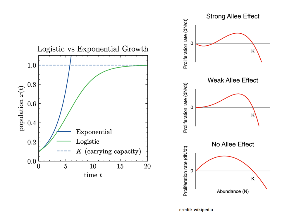
We now analyze a saturated growth model. Let be the population size, the intrinsic growth rate, the carrying capacity.
We start from the per-capita growth rate (proportional growth):
We then add a limited resources constraint: per-capita rate decreases with .
Intuition: the term limits the exponential growth up to .
The close form solution brings to:
In the logistic growth, if we consider , we obtain two equilibria:
- : unstable.
- : stable
The MSY (maximum sustainable yield) is obtained where .
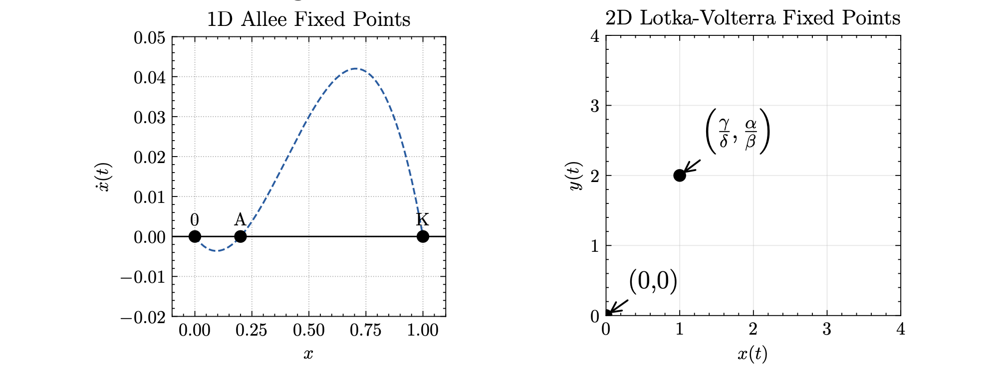
The Logistic Growth Differential Equation [Video]We now consider the Allee Effect, modelling the fact that, a low density, individuals struggle to grow. The model then becomes:
where the term models the critical density. The growth rate is then:
In the Allee dynamics, there are three equilibrium:
- and are stable
- is an unstable equilibrium
Indeed, if the population declines to , otherwise it grows to .
2.2 Fishing/Harvesting Model
We now consider a harvesting function , representing the rate at which a resource is removed from the population.:
- represents the stock(fish population)
- represents the effort (boats, manpower)
- represents the outflow of resources (catch per unit time)
Then we have:
At the equilibrium:
If we set , the equilbrium is given by .
Multiple cases possible:
- : above the MSY extinction.
- maximum yieldl, but not maximum risk.
- two intersections:
- the lower one is unstable, the upper one is stable.
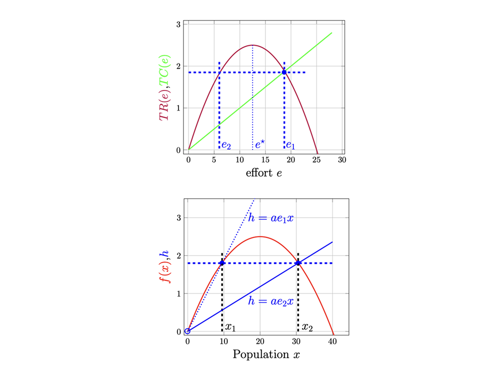
If we instead consider the harvesting function proportional to effor and resources (intuition: If the stock or drops, your harvest naturally drops - assuming effort the other stays the same- preventing accidental extinction better than a fixed quota because the "drain" slows down automatically as the population decreases):
the two equilibria are:
- (positive and then stable only if )
2.3 Growth Models: supply and demand determine price
In this case, the harvesting function is not fixed, but market driven.
- demand is decreasing in price
- supply is increasing in price and stock .
The market clearing is obtained as: and the equilibrium price :
The harvesting function becomes then a function of stock:
Then, since the stock is "consumed" by supply, that is equal to the harvesting function, We can the model the stock dynaimics as:
We now consider the profit function of a firm, given by:
with , wage effort; and revenue , with .
If we plug the previous equilibrium in the profit function and we set , we obtain:
- market entry as long as increases
- : excess profit, entry
- : profit further increases
- : proif decreasing but still .
- : no profit, not entry.
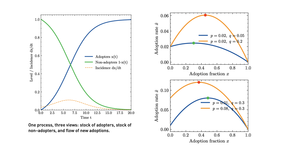
3.1 Common Source Diffusion
We start by analyzing a simple model with:
- representing the fraction adopted
- only external push
- No initial adopters: .
- adoption hazard
- share of non-adopters
The analytical solution is:
We clearly that this model is linear in (the logistic is instead quadratic) and it is always concave, with adoption slowing down as .
If we instead want to find the time to reach a target, we simply set:
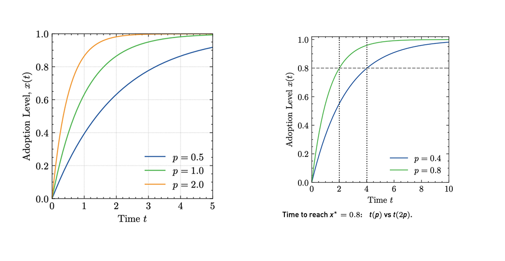
3.2 Bass Diffusion
In this model, each nonadopter is influenced by twho channels: adoption (as in the commono source one) and imitation or world of mouth, expressed by the term , increasing in :
Two special cases in this model:
- commono source model
- pure imitation, needs to start.
However, note that the Bass Model requires strong assumptions:
- adoption only driven by direct persuasion ( and )
- homogeneous population, no spatial or network effects
- no threshold dynamics and no critical mass modeled
- no economic ingredients (prices, preferences etc etc)
and strong limitations too:
- at the final state: with no reversal
- the model cannot capture competition, substitution or churn.
3.3 SIRS Models
Bass is an example of spreading model, epidemic models (SIRS) are the canonical toolkit for this scenarios.
We start by analyzing a SI model :
if we add a recovery rate and infection duration , we obtain a SIR model:
where is the recovery rate. We can define the Basic Reproduction Number as the number of infected from one person in a fully subscettible population as:
In this case, we have an early growth if and only if .
The effective reproduction number is then . The spread slows down and eventually stops when:
(since and ).
Intuition: once individuals are immune (recovered or vaccinated), each case generates less than one new case on average and infections dies out.
Finally, a SIRS model introduces a waning immuunity that vanishes at rate .
The end state is non trivial and it is given by the vector .
3.4 Complex Contagions on a graph: a formal setup
We consider a network , with noted and edges .
- each node ( non-adopter, adopter)
- adoption threshold
- neighborhood
The threshold rules says:
Intuition: node adopts if or more neighbors are adopters.
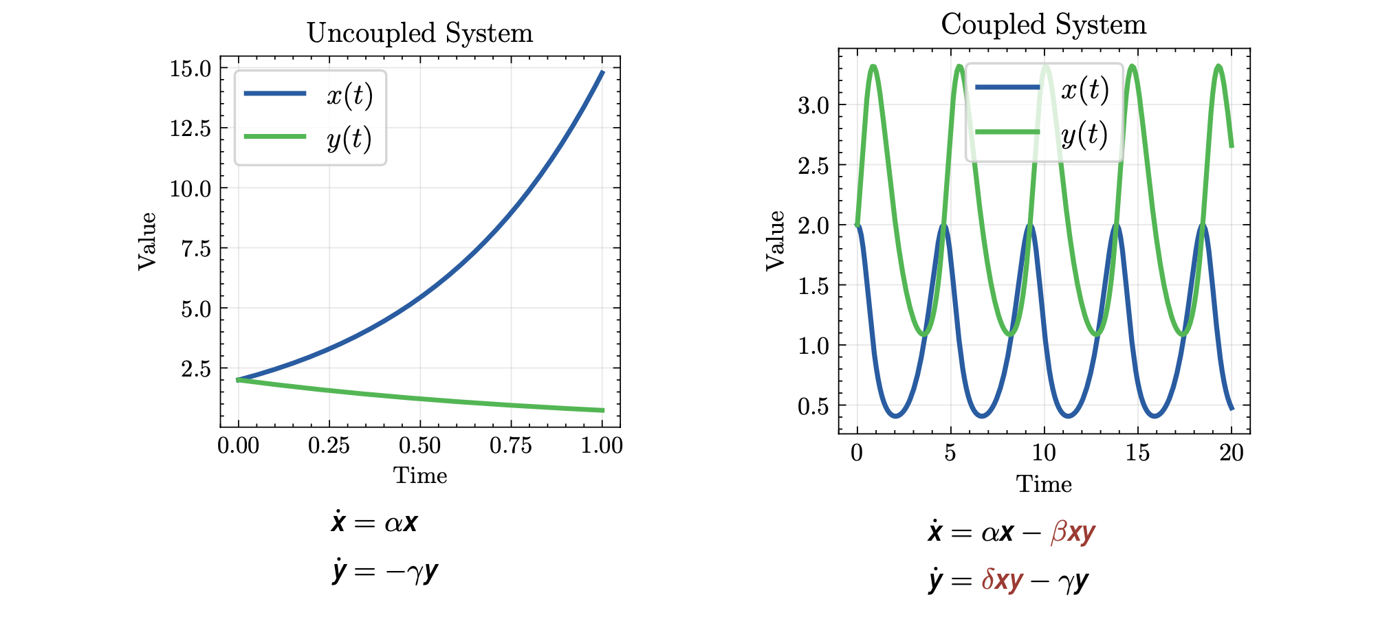
4.1 Coupled Dynamics: Lotka-Volterra Predator-Prey Model
Coupled dynamics are needed when two (or more) variables evolve together, leading to cycles, attractors and repellors. Common examples are predator and prey in biology, susceptible and infected in epidemiology, employment and wages in economics. In formulas, we can write:
The analysis of this systems comes from the classification of fixed points and stability, both analytically and numerically.
We start by analyzing the Lotka-Volterra Predator-Prey Model, representing the interaction between two species:
- : preys (hares)
- : predators (lynx)
Predator-Prey Population Models || Lotka-Volterra Equations [Video]
In isolation we know that:
- prey reproduces exponentially,
- predators die out: .
But, if together in the same ecosystem:
- interaction remove prey at rate
- interaction yields predators growth at rate .
resulting in the following coupled system:
We now show the procedure determine fixed points. We start by setting the following to find the equilibrium (fixed points :
In the case of the LV model we have:
resultig in:
In general, the number of roots will depend on and :
- Zero: no equilibria
- One: unique equilbrium
- Finite number : several isolated equilibria
- inftyinitely many: whole x-axis equilibria
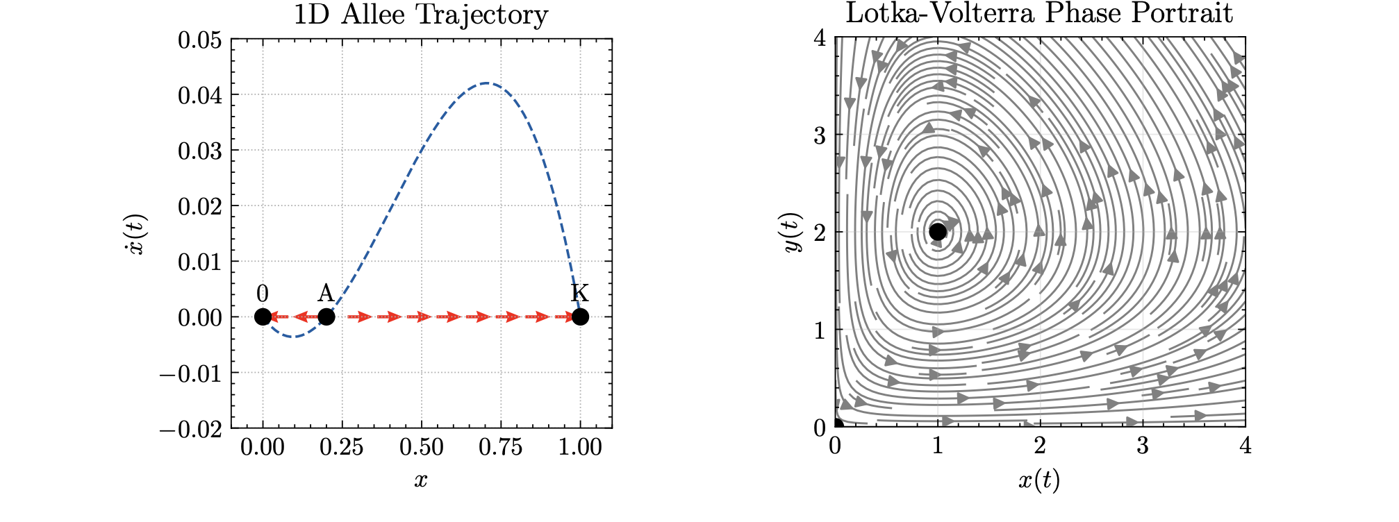
Note that, in higher dimensions, understanding stability and trajectories become more complicated that in the simple 1D case.
To visualize the trajectory of the system, a common approach is to numerically solve the ODEs with initial condition chosen and then run a series of simulations. From the plot, we should then be able to clearly see if the trajectories are converging, diverging or staying in rotation around the fixed points.
Then, at a fixed point, a non-linear system can be approximated by a linear one. Define perturbations as:
and, thanks to Taylor expansions, we end up in the dynamics for small perturbations:
The eigenvalues of Jacobian tell us whether perturbations grow, decay or oscillate. In the 1D case, we had that:
- if : perturbations decay (stable)
- if : perturbations grow (unstable)
The same applies to the 2D case. We consider , where is a costant vector.
Then we plug , resulting in:
We can clearly see that the eigenvalues of describe how small perturbations evolve.
Recall that to compute the eigenvalues of we can simply write and solve the characteristic polynomial:
leading to the following solution:
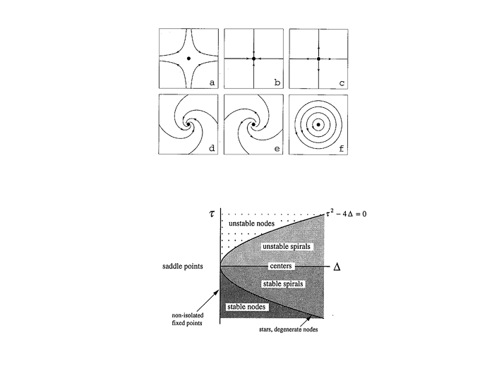
The classification of the fixed points can be done analytically depending on the characteristic polynomial:
- (a): Saddle: . are real and have opposite single
- (b,c): Stable and Unstable Nodes: and (stable with ). Also known as attractors and repellors, are real and have the same sign.
- (d,e): Stable and Unstable Spiral: and (stable with ). Also known as attractive focus and repulsive focus, are complex.
- (f): Center: and . are complex with zero real part.
Example: Stable/Unstable Spirals or Center in the Lotka-Volterra Model.
We consider the following model:
Explicitily computing the Jacobian:
we then find fixed points:
and we evaluate them at:
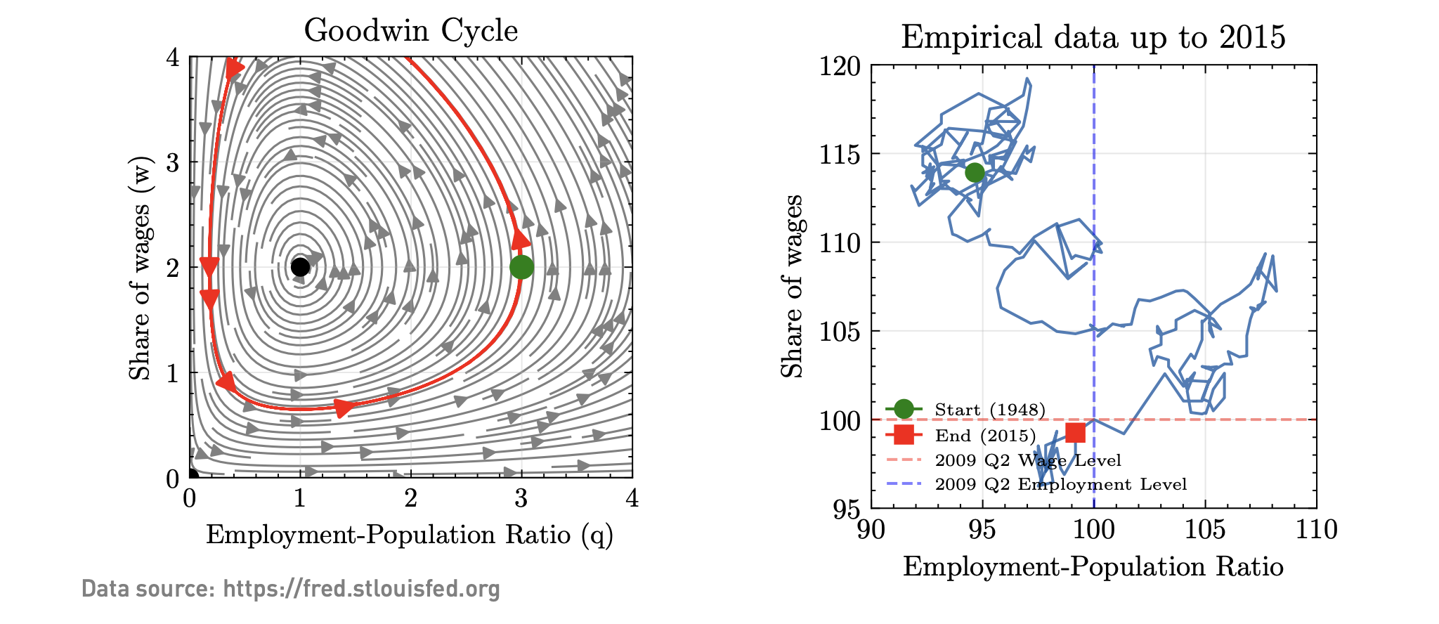
4.2 Coupled Dynamics: Goodwin's Model (1967), Cycles in Employment and Wages
The Goodwin's Model [Wikipedia]This model comes from a simple observation: economies often show recurrent cycles.
Booms cause high employment, so workers gain bargaining power, then wages rise, wage share of outpus increases as well. As a consequence, profits fall, investment slows and growth stalls.
Employment then falls, weakening workers' position, wages stagnate or declinde, profits recover and growth resumes.
Goodwin's idea is to model class struggle dynamics with similar equations used for predator-prey cycles.
We then consider two state variables:
- : employment ratio (jobs over the population) - analogy with the prey population
- : wage share (workers' share of output) - analogy with the predator population
The qualitative cycle logics says that:
- bargaining power
- profits investment
- wage pressure profits
Formally, if we consider the following variables:
- employment ratio
- wage share
- total output (GDP), with capital-output ratoi such that:
- capital stock (invested at: )
- employed labor
- total labor force, growing at rate .
- labor productivity, growing a rate .
- real wage, following the Philipps Curve with:
and parameters .
We then differentiate the employment ratio and the wage share:
Putting toghether, we have the Goodwmin's System:
Simplifying, we get:
The intuition, very similar to the previous predator-prey model, is that workers and capitalists are two interacting groups. Workers indeed seek higher wages, capitalists seek higher profits. These opposing objectives create a self-regulating cycle, neither side "wins" permanently but they co-move in economic cycles.
From an economic point of view:
- Growth-recessions cycles are endogenous without external shocks
- Booms (high ) are the beginning of slowdowns (rising ) and viceversa
- The neutral center is not robust, small modifications destroy cycles.
5.1 Discrete Dynamics: Cobweb Plot
There are several reason behind why we should discrete time dynamics:
- decision timing: firms and individuals set prices/output quarterly or at fixed intervals
- institutional calendars: central banks and governments meet on fixed dates
- contracts and billing: loans, rent and utilities are paid monthly or similarly
- observed data: GDP, monthly unemployments, annual reports etc etc...
To start with discrete time dynamics, we define the difference equation, representing how the next state depends on the previous:
The evolution if then given by the repeated application of :
To visualize this, we usually use Cobweb Plot, showing the evolution of the discrete rule.
- Start with a initial value .
- Move vertically till the blue line representing and find .
- Move horizontally to the diagonal and find .
- Repeat with and iterate.
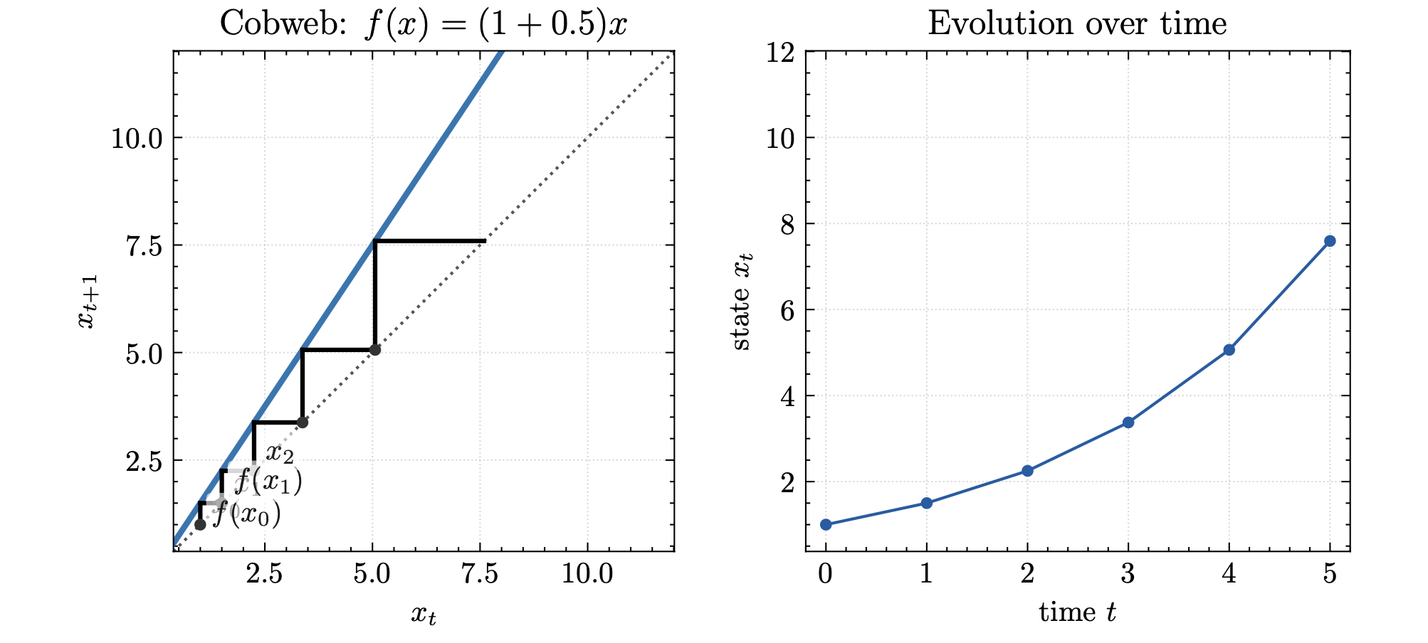
Each update defined a sequence:
when crosses we have fixed points .
Note that the sequence may cycle set of points (periodi orbits) or may be aperiodic (chaotic) deterministic, but not repeating.
To determine the fixed points, we have to find such that .
We then consider, as usual, the deviation from the fixed point:
and we linearize around :
if we then iterate times we obtain:
To determine if it is stable or not, we simply look at:
- attracting
- repelling
- monotone
- alternating
5.2 Discrete Dynamics: Saturated (Logistic) Growth
We previously analyzed the continuous-time logistic growth as:
if we apply the Euler discretization as:
we can then write:
if we define :
We now determine fixed points:
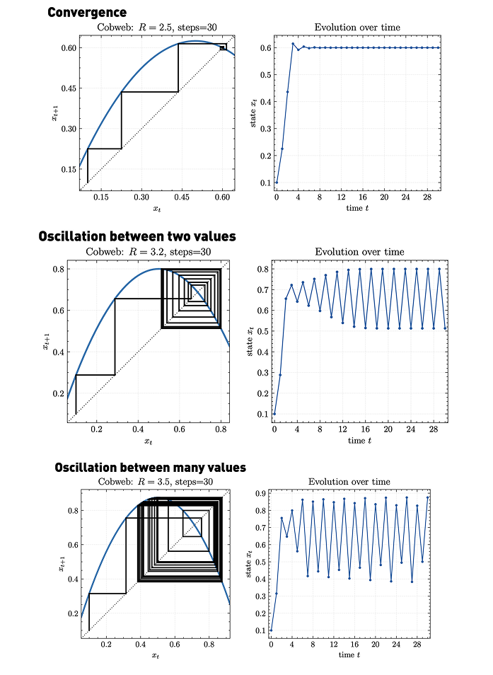
we now apply the stability condition on the first derivative :
- if then and the fixed points attract
- at : flip bifurcation (fixed points becomes repelling: stable 2-cycles).
Intuition: As long as the growth rate is between 1 and 3, the population settles down to . At exactly , the slope becomes . This is the "tipping point": The system can no longer settle at a single number.
In the second period, if , the population starts jumping back and forth between two values, and , every period. The period-2 points solve , resulting in:
As in the first cycle, in the -cycle, we obtain stability is reached when: , that, for the -cycle rewrites as:
At the -cycle does another flip (stable 4-cycle, the population repeats a pattern of 4 different values)
For many periods, we now consider the value of where a -cycle first appears:
The sequence converges geometrically to
We then define the Feigenbaum constant as:
resulting in the Scaling Law for :
More on the Feigenbaum Constants [Wikipedia]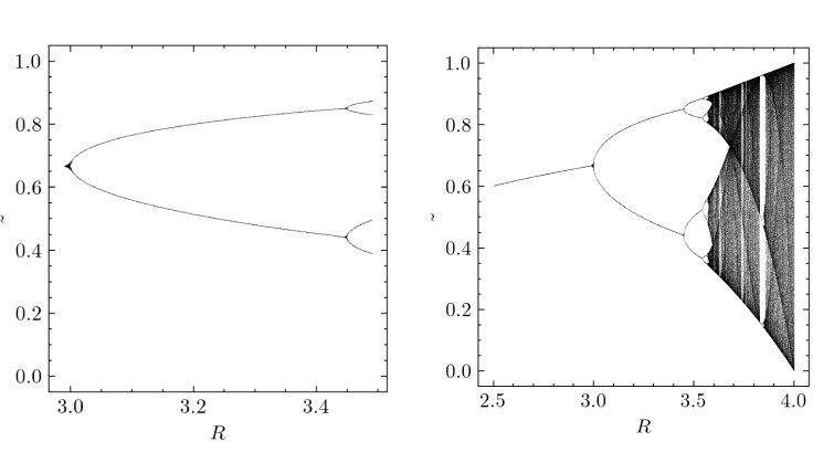
- For we can see a mixture of order and chaos: periodic windows reappe within chaotic bands.
- At we see fully developed chaos.
This is called deterministic chaos: once and are fixed, each step is predetermined, but long term behavior becomes unpredictable, because tiny differences in grow rapidly.
A deterministc system is then called chaotic when it shows:
- aperiodic long-run behavior (no fixed points or repeating patterns)
- determinism
- sensitivity to initial conditions
Note that, as we've seen, deterministic predictable. In non-linear systems, tiny errors or deviations can explode over time, therefore long term forecasts lose meaning.
6.1 Endogenous Cycles
In the economy, markets are rarely isolated (producers can switch between goods, farmers can sell domestically or abroad, energy and manufacturing costs increase etc, etc...) We start now from the simple Cobweb Model but allow producers to switch markets.
Each market has a ficed supplier share , with .
if we set the market clearing condition :
then we can find the Price-Update Rule:
At the equilibrium:
Note that larger faster response to equilibrium and then less stability.
We now consider costs and profits in each market. Each supplier earn , depending on price and total quantity:
assuming that cost increases with ouput:
we result in the following profit funtion:
Now we can see the coupled system as a sequence of events:
- The suppliers produce , with is the probability of choosing a market depending on the profits:
where is the intensity of choice (rationality).
- Prices adjust to clear each market:
- Profits are realized
- Suppliers update market choice for the next period
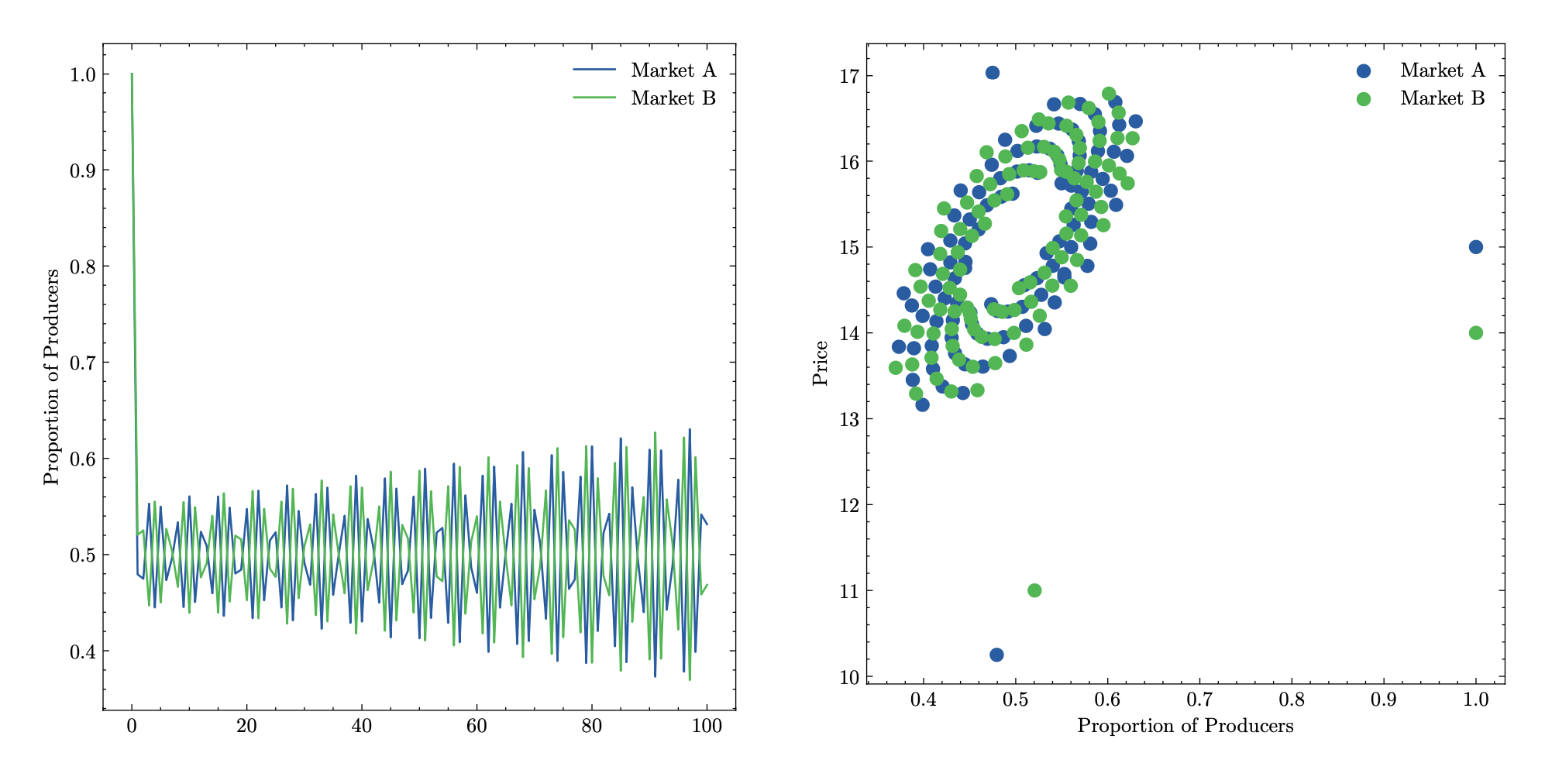
Be aware that, in the following plots, the x-axis is different!
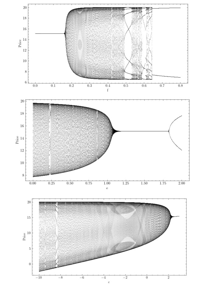
To understand if it is chaos or just complex, we can perform a FFT test.
A time series can be indeed seen as a mix of pure waves. We then apply the Fourier Transform to understand how much of each frequency is present.
Plotting then gives a spectrum:
- peaks in the spectrum represents cycles (not chaotic)
- no clear peaks in the spectrum implies that there's not a dominant rhythm.
In general, we can conclude about endogenous cycles that:
- Volatility is structural and it is amplified by a large supplier share in the market, faster switching intensity and excessive supply response (low ).
- Cycles create deadweight loss: mis-times investment and wasted inventory/resources.
- Coupling transmits fluctuations across markets.
6.2 Endogenous Cycles: Kaldor Model (Business Cycle)
We now model a 2-player model with:
- Household that can either consume or save:
- Capicalists that can either consume or invest:
- Savings fund investments: via banks
- At equilibrium: .
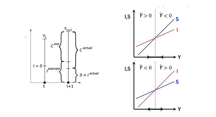
Starting from the setup we have:
- Households consume and save .
- Firms plan investment based on the expecteded consumption
- in reality, .
- The gap shows up as:
- The firm reacts:
- If overproduction, cut output
- If underproduction, expand output
- Leading to the dynamic rule:
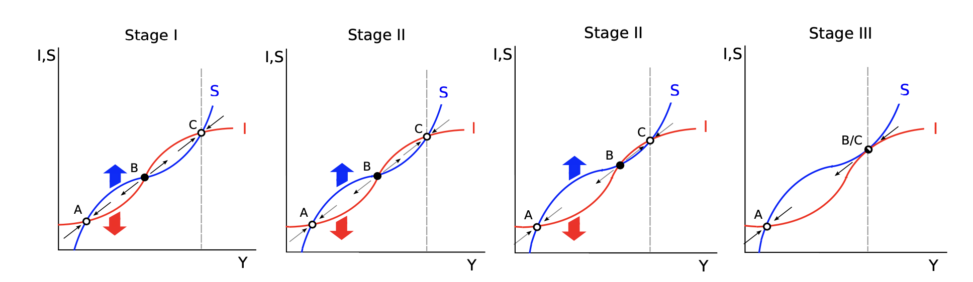
we can then incur in two scenarios:
- if has a steeper slope than (at the right of the equilibrium and at the left ): stable equilibrium.
- if has a steeper slope than (at the right of the equilibrium and at the left ): unstable equilibrium.
Kaldor's idea (1940) is that the saving and investment curves are not linear:
- For middle ranges of income, apperas linrar, but with larger income people save a larger proportion of their investment and at lower incomes they save drastically less .
- Similarly, is linear only in the middle range: at lower there's little incentive to invest and at a very high there are rising costs and borrowing constraints (so grows slower).
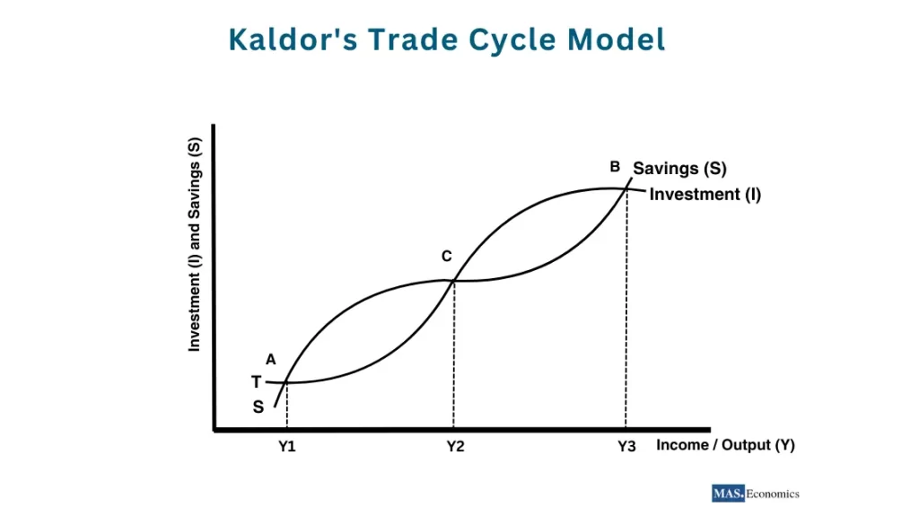
- Note that both can be "S" shaped.
- Note also that, at low income levels , the savings curve drops below the horizontal axis, representing negative savings, rather than approaching zero asymptotically.
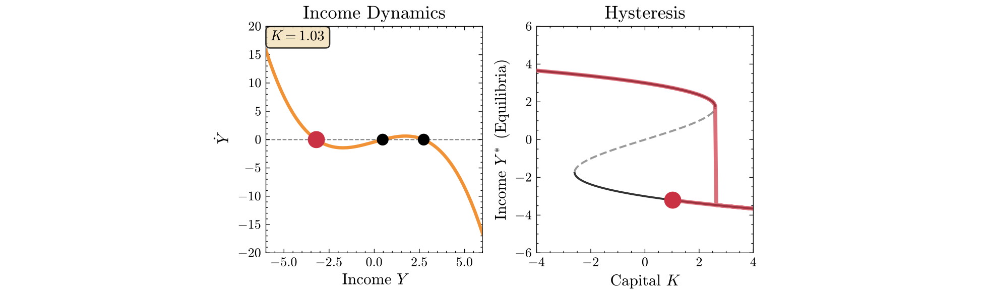
So far, we treaded investment and savings as a function of the output, in reality, they also depend on the capital stock , that accumulates through investment and declines thorugh depreciation, reflecting past investment decisions. We can then write (Kaldor Model):
In this model, if we assume that is set externally, we have 3 equilibria: two are stable (A,C) and one unstable (B)
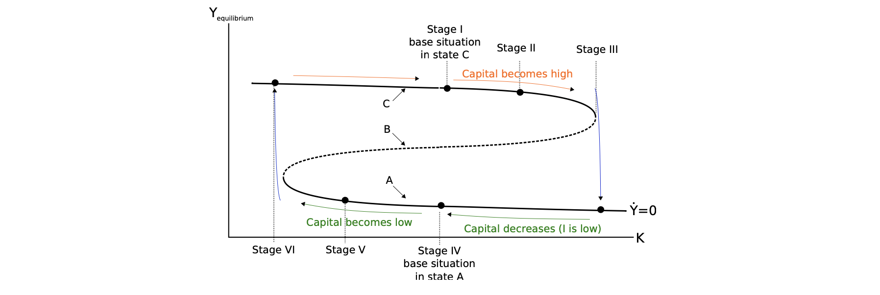
then introduces a hysteresis cycle: the equilibrium state is path dependent.
- an economy starts on the high branch (high income).
- as increases, the economy moves to the right along the top red line.
- eventually, it reaches the "knee" or the edge of the cliff.
- if increases past this point, the economy crashes down to the low branch.
- once it falls to the bottom level, it remain stuck in the low-income state
- to get back to the high-income state, the economy jas to decrease to move way to the left on the graph and to find the other "knee" where the system jumps up.
Note that, since no equilibrium satisfies , the economy follows a closed cycle.
If we then allow to have its own dyncamics, we have the full Kaldor Model.
The economy then moves around the unstable equilibrium: the interaction of fast and slow creates endogenous cycles. Note that represents the speed of the economy, while the speed of capital and they both shape the curvature of the cycles.
7.1 Introduction to Networks
A network (graph) is tuple :
- : the set of nodes (vertices)
- : set of links (edges)
- : all possible ordered pairs
We use the direction convention:
A network can be stored as a adjacency matrix :
- Rows represent the sources (outgoing link)
- Column represent the targets (incoming links)
A network is directed if
In a weighted network links have a numerical strength. A function assigns a weight to each link and the adjacency matrix becomes real-valued.
A link of the form is called self-loop and it appears in the diagonal entry (economically, it represents the self-dependence or internal feedback).
A node's degree is the number of links connected to it (economically: they represent connectivity of a node). Also, in a directed network, we can distinguish:
- indegree : number of incoming links
- outdegree : number of incoming links
In a weighted network, a node's strength sums the weights of its connections:
In a unweighted network, a node's strength is a simple in-and-out degree count.
A path between nodes and is a sequence such that:
- each pair
The path length is, of course, the number of links.
The distance between two nodes is the length of the shortest path connecting them. If no path exists: .
The network diameter is the longest shortest path in the network.
The average shortest path length measures typical separation.
A network is connected if for all .
Connected components are connected subgraphs .
The largest component is the giant connected component (GCC) if .
Degree centrality of a node is the number of its direct links (economically it measures the connectivity as exposure/access to partners, lenders, clients or other nodes)
Betweeness centrality counts how often node lies on the shortest paths between others:
where is the shortest path through . In the normalized form, we also write:
where is the total number of shortest shortest paths .
8.1 Diffusion on Networks
We define diffusion as flow across links (in the two nodes case). Suppose we have two noes connected by one link: the flow is then proportional to the difference between two states. We can then write an ODEs for the nodes:
with the conservation constraint: and parameter with unit .
The previous ODEs bring the convergence to stationarity:
If we generalize this to a graph and define an ODE for every node:
with the conservation contraint: (average preserved).
From the aggregate network, we can study the node-level dynamics. Consider a node :
(For example, we could choose modelling a Bass diffusion and then the rest to model the network)
To study better the behavior of the network, we proceed by computing the Laplacian Matrix.
Consider degrees and .
The Laplacian Matrix is and we can then rewrite the ODEs compactly:
We now proceed with the spectral decomposition of the Laplacian Matrix.
Recall: the spectral decomposition of a generic diagonalisable matrix is , where is the eigenvector matrix and the eigenvalues diagonal matrix.
Visualize Spectral Decomposition [Video]Define as the eigenvectors, forming an orthonormal basis. Then we write: with .
Define then the projections (intuition: are the time-dependent coefficients showing how "strong" each pattern/eigenvector is at time ) and then:
Now plug into . Since is an eigenvector, multiplying it by the matrix is simple: , resulting in:
Because eigenvectors are linearly independent, we can splits the big matrix problem into separate problems:
This is the decoupling of the ODE: each evolves indepedently and we can solve each one, resulting in:
and, finally, in:
- the term with the smallest eigenvalue may have and therefore this one does not decay, representing the final equilibrium state ( average value across the network)
- the terms with large eigenvalues decay very fast.
- the terms with small eigenvalues decay slowly.
Now we want a single number to measure how far we are from stationarity.
- we start by computing the average:
- we compute the per-node deviation: .
- we compute the network deviation and track it over time:
In fact, after some algebraic manipulation, we can see that decays with rate .
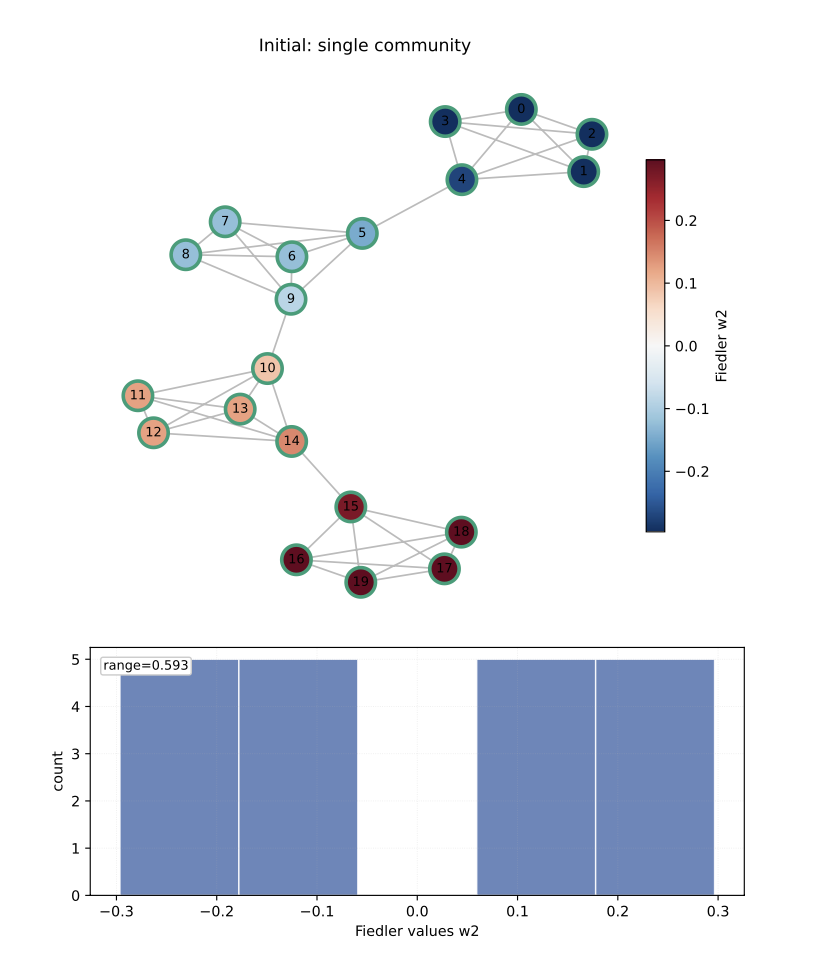
So, if we consider a connected network, the second-smallest eigenvalue is called the algebraic connectivity (also known as Fiedler Vector) and determines how fast or slow diffusion is. The smaller , the harder is to cross the network (capturing how well-connected a network is).
If we now consider a network with two disconnected components:
- each block in the matrix is another Laplacina Matrix
- each has a trivial eigenvalue with eigenvectors and (depending on the component size)
Therefore, has two zero eigenvalues, so and the network is disconnected.
If we consider then the deviations , we can simply derive that deviations follow the same linear system:
and, therefore, face the same dynamics:
of course, as before, approach to stationarity is determined by eigenvalues of . Note that, however, (it's mean free!).
Spectral Graph Theory For Dummies [Video]Introduction of algebraic connectivity and Fiedler vector [Video]
9.1 Community Detection: Dirichlet Energy, Rayleigh Quotient and Network Bisection
Considering what we said in the previous chapter, we can go on studying networks. We start by defining the energy of a single edge for a node state as:
- the energy penalizes disagreement across a link: it's zero if neighbors agree.
- it is large on weak links where values "jump" between nodes.
If we then sum over all edges, we obtain the Dirichlet Graph Energy:
Then, for any non-zero vector of nodes, we can define the Rayleigh Quotient , representing how well the state (or vector of nodes) fits the network, i.e. how uneven values are across linked regions (smooth profiles show small )
At the numerator we have the total edge energy, large if neighbors differ a lot, at the denominator a scale normalization.
Also, we know that:
intuition: is the vector that minimizes the Rayleigh quotient.
Now, to identify communities within a network, consider the following two sets:
intuition: minimizes tension across edges, leaning to a smooth split across the weakest connection.
We can then apply this procedure recursively to find finer communities. Common stopping criteria are: max depth and min size. Note that bisection using the fiedler vector cannot detect more than two communities at once.
Example: Spectral bisection algorithm in Python:
def spectral_bisection(G):
   L = laplacian(G) # L = K - A
   w2 = second_eigenvector(L) # Fiedler vector
   Spos = {i for i in G.nodes if w2[i] > 0}
   Sneg = set(G.nodes) - Spos
   return Spos, Sneg
def recursive_spectral(G, depth=0, max_depth=3):
   if depth == max_depth or len(G) < 3:
       return [set(G.nodes)]
   Spos, Sneg = spectral_bisection(G)
   return (recursive_spectral(G.subgraph(Spos), depth+1, max_depth)
         + recursive_spectral(G.subgraph(Sneg), depth+1, max_depth))
9.2 Network Eigenvector Centralities
We saw in the last chapters that degree counts links, but not all links are equal. Indeed, a connection to an important node should matter more than one to an unimportant node. Inutition: each node's importante should depend oon the importance of its neighbors.
To compute then the centrality of a node, we can start with a guess and repeatedly update it using the network structure.
- we start with initial centrality (all equal to one)
- we sum all the neighbots centralities with const. of proportionality.
or, equivalently:
This reduced to the eigenvector equation :
with the leading eigenvector giving the eigenvector centrality.
- we repeat this procedure until the vector of centralities converges.
Intuition: high centrality comes from many neighbors (quantity) and/or a few but very central neighbors (quality). Also, note that eigenvector centrality works best for connected, undirected networks.
Also, note that root nodes have no incoming edge, so it gets , by consequence, any node that is pointed to only by the root also gets . (the zero propagates backward through the graph: nodes reachable only from roots inherit zero centrality).
9.3 Katz and PageRank Centralities
To fix the previous problem of the propagation of the zero, Katz Centrality fives each node a small , so importance can start everywhere:
Intuition: adds endogenous centrality. Note: choose to ensure convergence.
The problem in this model is that an high centrality node can pass large score to many neighbors. To fix this, the PageRank algorithm dilutes a node's contribution by its out-degree:
PageRank it was firstly introducted by Google to rank web pages, widely used because it downweights mega-directories that link to millions. Google famously used .
In matrix form, the PageRank model rewrites as:
note that:
- does not affect the results (just scaling)
- must be smaller than the largest eigenvalue of .
10.1 Strategic Network Formation
Given a formed network, we now model how agents can influence and modify the network. Agents can be representes as noded on a network with a utility based on their position:
The social welfare is then:
A network is socially efficient if . (intuition: no other feasible network yields higher total welfare).
Pairwise stability occurs when:
- no agent wants to cut an existing link
- no agent pairs wants to add a new link
10.2 The Connections Model (1996)
In this model, agents are nodes in an undirected network, links give access to information and benefits come from both direct and indirect neighbours, with the following utility:
where is the shortest-path disstance between , is is not reachable, represents then the benefit decay per step and each link costs .
We now analyze the welfare of a complete graph , where every node is linked to all others. For node , we have the following utility:
resulting in the following total welfare:
A similar approach can be applied to the Star Graph :
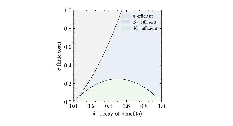
We can now compare when is better than the empty network:
and when is better than :
In these models, we often incurr in externalities: actions that change other's utility but whose effects the decision kamer does not internalize.
Positive externalities include new links make others better (shorter paths) but, since agents do not take these benefits into account, the result is under connected network (too few links in equilibrium).
Negative externalitiea include that links can harm others _(diluiting resources), resulting in a over connected network.
To compensate externalities, we can introduce side payments in the moel to share .
The idea is that, if a link increases , endpoints can transfer payoffs, so losers can be compe sated by winners:
10.3 The Co-Author Model
Nodes represent researchers, links are co-autorships.
- A collaboration creates value for both but...
- each researcher has limited time
- a collaborator with many co-authors is less focused
- adding a link reduced efficiency for all other projects.
- Negative externality: when a researcher takes another project with someone else, it reduces the value of existing collaborations.
Let the number of co-authors (degree) of researcher :
We can clearly see that, if increases : every one of 's projects becomes less valuable.
In this specific model, welfare is maximized when each collaboratoin has 2 fully focused researchers:
The efficient network (maximum welfare) is a set of disjoint pairs (for even ).
11.1 Dynamics of Strategic Network Formation
Knowing which networks are efficient or stable doesn't tewll us which networks actually emerge. Networks grow through sequence of local decisions, creating a dynamic system where path-dependence can arise.
In the last section, we have seen that several networks are stable, but we assumed the cost per link constant. In reality, maintaining more links becomes more expensive: to account for this we introduce quadratic costs .
the marginal cost of adding one link is then:
Intuition: first links are cheap, link costs grow with degree.
Under linear costs, we have seen star-like or core-periphery structures. With quadratic costs highest degrees are much smaller and networks look more "egalitarian" (no super hubs). This happen because, with high marginal costs, they stop adding links earlier.
To simulate the network formation game, please use this very cool tool by Luca Verginer!We consider now a potential network with nodes, with possible links and possible networks.
In this scenario, pairwise-stable networks are a tiny subset.
Our process is a slow, myopic search in a gigantic space: therefore, we chanfe one link at time with the following rule:
- pick a random pair
- add the link if both gain
- delete the link if one gains
In simulation, this long process shows up as:
- long transients with very slow convergence, if at all
- oscillations with the number of links and welfare fluctuate.
With large, also the number of constraints to reach pairwise-stability grow superlinearly in .
Key takeaway: in large economic networks, the ongoing dynamic is more important the the (unreachable) equilibrium.
11.2 Spatial Connections Model.(Jackson and Wolinsky, 1996)
So far, networks lived in an abstract place, but in reality and in many economic networks, agents have a location. Empirically, we see:
- strong local connectivity (public transports)
- a few long range link (airports)
We now try to extend the connection models to take into account to model:
- easier access to nearby agents
- more expensive long-range links
We then consider than eachn ode has a position and is the distance between , then:
Intuition: geography acts as an extra hops in the network, increasing the effective distance exponent.
- Closer neighbours have smaller exponent and larger benefits
- distand nodes have small benefits unless we create shortcuts.
In the simple case, with two isolated nodes , link forms if:
is also defined as the critical distance .