AR, VAR and BVAR in Macroeconomic Forecasting

These notes are freely taken from my course Methods for Macroeconomic Forecasting, by Samad Sarferaz at the KOF Swiss Economic Institute.

For a more practical perspective , I refer to the final part of this article, where I provide a short overview of my course project and the GitHub Course Repository.

Index:

Autoregressive Model (AR)
Vector Autoregressive Model (VAR)
Bayesian Vector Autoregressive Model (BVAR)
Macroeconomic Forecasting Project (R)
Bibliography

Introduction to AR, VAR, and BVAR Models

Time series models are essential tools in macroeconomics , where variables evolve over time and influence one another.
To forecast them, most widely used are the Autoregressive (AR) , Vector Autoregressive (VAR), and Bayesian Vector Autoregressive (BVAR) models.

AR is the simplest one and captures persistence in a single variable: the intituition is that its past values affect the current one.
VAR extends this idea to multiple variables, capturing the influence of each on the others.
BVAR applies Bayesian shrinkage to VARs, improving forecasts when data are limited or when there are many variables (reducing overfitting).

Below, you will find a more detailed overview of these methods.

Autoregressive Model (AR)

An AR model of order $p$ , denoted AR( $p$ ), is written as:

y_{t} = c + ϕ_{1} y_{t - 1} + ϕ_{2} y_{t - 2} + \dots + ϕ_{p} y_{t - p} + ε_{t},

where:

$y_{t}$ = value of the variable at time $t$ ,
$c$ = intercept or drift term,
$ϕ_{i}$ = autoregressive coefficients,
$ε_{t}$ = white noise error term, $ε_{t} \sim (0, σ^{2})$ .

The model implies that current observations depend linearly on a finite number of past observations.

The simplest case, AR(1), is:

y_{t} = c + ϕ y_{t - 1} + ε_{t} .

If $∣ ϕ ∣ < 1$ : the process is stationary and mean-reverting.
If $ϕ = 1$ : the process has a unit root (random walk).
If $∣ ϕ ∣ > 1$ : the process is explosive.

The mean and variance of a stationary AR(1) are:

E [y_{t}] = \frac{c}{1 - ϕ}, Va r (y_{t}) = \frac{σ ^{2}}{1 - ϕ ^{2}} .

For the AR( $p$ ) process to be covariance-stationary, all roots of the characteristic polynomial must lie outside the unit circle:

1 - ϕ_{1} z - ϕ_{2} z^{2} - \dots - ϕ_{p} z^{p} = 0, ∣ z ∣ > 1.

Stationarity implies that the series has:

Constant mean and variance,
Autocovariances depending only on the lag, not on time.

If not stationary, we often difference the series to induce stationarity.

Estimation and Forecasting

The parameters $ϕ_{i}$ and $c$ can be estimated by Ordinary Least Squares (OLS) since the model is linear in parameters:

\hat{ϕ} = (Y^{'} Y)^{- 1} Y^{'} y,

where $Y$ contains lagged values $[y_{t - 1}, y_{t - 2}, \dots, y_{t - p}]$ .
Alternatively, one can use Maximum Likelihood Estimation (MLE) under Gaussian errors.

The one-step ahead forecast can be computed as:

\overset{y}{^}_{t + 1∣ t} = c + ϕ y_{t} .

and the multi-step ahead for an horizon $h$ as:

\overset{y}{^}_{t + h ∣ t} = μ (1 - ϕ^{h}) + ϕ^{h} y_{t}, where μ = \frac{c}{1 - ϕ} .

Note that the forecast converges to the long-run mean $μ$ as $h \to \infty$ , but forecast uncertainty grows with $h$ as errors accumulate.

We now introducte the Autocorellation Function ACF that, for a stationary AR(1) is defined as: For a stationary AR(1), :

ρ (k) = ϕ^{k},

Clearly, autocorrelation decays geometrically with the lag $k$ .
This property makes AR models suitable for data that exhibit exponential decay in correlation.

Economic Interpretation

In macroeconomics, AR models are often used as benchmark forecasting tools for individual variables:

GDP growth, inflation, or unemployment rates are often modeled as AR(1) or AR(2) processes.
The persistence parameter $ϕ$ captures how strongly the past influences the present.
Shocks $ε_{t}$ represent unexpected innovations or disturbances (e.g., policy, technology, or demand shocks).

Even though AR models ignore cross-variable interactions, they remain valuable for baseline forecasts and for testing more complex models like VARs or BVARs. But... AR comes with some limitations:

Ignores relationships between multiple variables (univariate only).
Cannot capture structural changes or regime shifts.
Non-stationary series require differencing or transformation.

Vector Autoregressive Model (VAR)

A Vector Autoregressive model (VAR) is a multivariate generalization of the univariate autoregressive model (AR).
It captures dynamic interdependencies* among multiple time series variables, all influencing each other over time.

Formally, for an $n$ -dimensional vector of variables:

y_{t} = y_{1 t} y_{2 t} ⋮ y_{n t},

a VAR of order $p$ (denoted VAR( $p$ )) is defined as:

y_{t} = c + A_{1} y_{t - 1} + A_{2} y_{t - 2} + \dots + A_{p} y_{t - p} + u_{t},

where:

$y_{t} \in R^{n}$ is the vector of endogenous variables,
$c \in R^{n}$ is a vector of intercepts,
$A_{i} \in R^{n \times n}$ are coefficient matrices,
$u_{t} \sim (0, Σ_{u})$ is a white-noise innovation vector with covariance matrix $Σ_{u}$ , representing the unpredictable part of the process.

A VAR( $p$ ) is covariance-stationary if all roots of the characteristic equation lie outside the unit circle.

det (I_{n} - A_{1} z - A_{2} z^{2} - \dots - A_{p} z^{p}) \neq = 0, for ∣ z ∣ \leq 1.

If the process is stationary:

The unconditional mean is $μ_{y} = (I_{n} - A_{1} - A_{2} - \dots - A_{p})^{- 1} c .$
The system has finite variances and autocovariances.

If not stationary (unit roots present), one often uses differenced VARs or Vector Error Correction Models (VECMs) for cointegrated data.

Estimation and Forecasting

Each equation in the VAR can be estimated OLS independently because all right-hand-side variables are the same in each equation.

Let:

Y = [y_{p}, y_{p + 1}, \dots, y_{T}]^{'}, X = [1, y_{t - 1}^{'}, y_{t - 2}^{'}, \dots, y_{t - p}^{'}] .

Then the model can be written compactly as:

Y = XB + U,

where:

$B = [c, A_{1}, A_{2}, \dots, A_{p}]^{'}$ is the matrix of coefficients,
$U$ is the matrix of residuals.

The OLS estimator is:

\hat{B} = (X^{'} X)^{- 1} X^{'} Y .

Once estimated, a VAR model can generate multi-step forecasts recursively.

For $h$ -step ahead forecasts:

\overset{y}{^}_{t + h ∣ t} = c + A_{1} \overset{y}{^}_{t + h - 1∣ t} + \dots + A_{p} \overset{y}{^}_{t + h - p ∣ t} .

Forecast Error Variance Decomposition (FEVD)

FEVD shows how much of the forecast error variance of each variable can be attributed to shocks (innovations) in each variable of the system.

In other words, FEVD helps answer: “How much of the variation in variable i is explained by shocks to variable j _over time?

Consider a reduced-form VAR(p) model:

y_{t} = A_{1} y_{t - 1} + A_{2} y_{t - 2} + \dots + A_{p} y_{t - p} + ε_{t}, ε_{t} \sim (0, Σ_{ε})

It can be written in its moving average (MA) representation:

y_{t} = μ + i = 0 \sum \infty Φ_{i} ε_{t - i}

where $Φ_{i}$ are matrices of impulse responses.

The h-step ahead forecast made at time $t$ is:

\overset{y}{^}_{t + h ∣ t} = E_{t} [y_{t + h}] = μ + i = 1 \sum h Φ_{i} ε_{t + h - i}

The forecast error is:

y_{t + h} - \overset{y}{^}_{t + h ∣ t} = i = 0 \sum h - 1 Φ_{i} ε_{t + h - i}

and its variance:

Va r (y_{t + h} - \overset{y}{^}_{t + h ∣ t}) = i = 0 \sum h - 1 Φ_{i} Σ_{ε} Φ_{i}^{'}

FEVD decomposes this total forecast error variance for each variable $y_{j}$ into the portion attributable to shocks in each variable $ε_{k}$ :

θ_{jk} (h) = \frac{\sum _{i = 0}^{h - 1} ( e _{j}^{'} Φ _{i} P e _{k} ) ^{2}}{\sum _{i = 0}^{h - 1} ( e _{j}^{'} Φ _{i} P P ^{'} Φ _{i}^{'} e _{j} )}

where:

$e_{j}$ : selection vector (1 in the j-th position, 0 elsewhere)
$P$ : matrix that orthogonalizes innovations (e.g., Cholesky factor of $Σ_{ε}$ )

Thus, $θ_{jk} (h)$ represents the percentage of the forecast error variance of variable $j$ at horizon $h$ explained by shocks to variable $k$ , providing a quantitative measure of dynamic interdependence and helping to identify most influential shocks.

Impulse Response Functions (IRFs)

IRFs quantifies the effect of a one-time shock in one variable on the current and future values of all variables, it answer “What happens to variable $i$ if we shock variable $j$ by one unit today?”

Since the innovations $ε_{t}$ are often correlated, we cannot interpret them as isolated shocks.
To obtain independent shocks, we perform orthogonalization:

ε_{t} = P u_{t}, Va r (u_{t}) = I

where $P$ is usually obtained via Cholesky decomposition of $Σ_{ε}$ .

Then, given the orthogonalized IRF:

Ψ_{i} = Φ_{i} P

we can define the response of variable $j$ to a unit shock in $u_{k}$ after $i$ periods is:

ψ_{jk, i}

IRFs represents therefore shows both short-term immediate effects of shocks and long-run persistent dynamics and equilibrium adjustment.

Bayesian Vector Autoregressive Model (VAR)

A BVAR is the Bayesian extension of the classical Vector AutoRegression (VAR) model.

The classical VAR assumes indeed that true parameter values exist, and the task is to estimate them as accurately as possible from the sample.

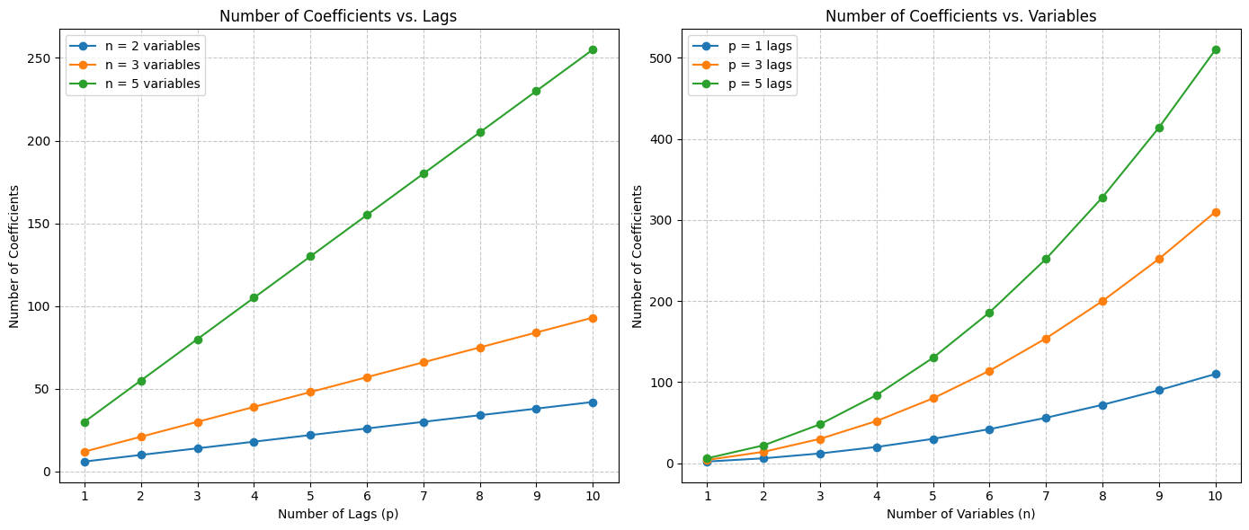
The main problem is that, as the number of variables $K$ and lags $p$ increases, the number of parameters to estimate grows quadratically.
For example, a VAR with 10 variables and 4 lags already has 400 coefficients to estimate, and that’s not even counting intercepts or covariances.

Number of coefficients in VAR

Problems of VAR

This leads to several practical issues:

Overfitting: the model adapts too much to the sample data
Parameter instability: small sample size leads to unreliable estimates.

leading traditional VAR models become unmanageable and statistically weak when the dataset is small but the system is large.

A BVAR mitigates this dimensionality problem by introducing prior information (the priors) about the model parameters.

Instead of estimating the coefficients only from the data, a BVAR combines:

The likelihood (what the data tell us)
he prior distribution (what we believe about the parameters before observing the data)

This combination yields a posterior distribution that balances data-driven evidence and prior beliefs.

In a BVAR, parameters are treated as random variables that have their own probability distributions.
This reflects the idea that we are uncertain about the true values.

The Role of Priors (Prior Distributions) and the Estimation Mechanism

The estimation procedure of a BVAR relies on the principles of Bayesian inference, where parameter uncertainty is explicitly modeled rather than ignored.

Let $Y = (y_{1}, y_{2}, \dots, y_{T})$ be the observed data and let the model parameters be $Θ = (A_{1}, \dots, A_{p}, Σ)$ .
The goal is to determine the posterior distribution $p (Θ ∣ Y)$ , which represents the updated beliefs about the parameters after observing the data.

According to Bayes’ theorem :

p (Θ ∣ Y) = \frac{p ( Y ∣ Θ ) p ( Θ )}{p ( Y )}

where:

$p (Y ∣ Θ)$ : Likelihood function , capturing the probability of the observed data given the parameters.
$p (Θ)$ : Prior distribution, giving information the parameters before observing the data.
$p (Y)$ : Marginal likelihood or evidence, serving as a normalizing constant.

Combining prior and likelihood yields the posterior:

p (A, Σ ∣ Y) \propto p (Y ∣ A, Σ) p (A, Σ)

So, in the BVAR, we obtain the followings

Parameters are random variables.
Output is composed by a posterior distributions for each coefficient $p (A_{ij} ∣ Y)$ .
Uncertainty is intrinsic to the model and explicitly quantified.
Forecasts integrate over parameter uncertainty: $p (y_{T + h} ∣ Y) = \int p (y_{T + h} ∣ A, Σ, Y) p (A, Σ ∣ Y) d A d Σ$
Estimation can produce full distributions, means, medians, or credible intervals.

In a BVAR, we are not looking for the true values of fixed parameters, but rather a probabilistic belief about them.

In many standard priors (e.g., Normal-Inverse Wishart), the posterior distributions remain in the same conjugate family (prior and posterior belong to the same probability family), which allows closed-form analytical solutions for posterior means and variances.

When conjugacy does not hold, simulation-based methods (Markov Chain Monte Carlo (MCMC) or Gibbs sampling) are employed to approximate the posterior.

Number of coefficients in VAR

Details in the Bibliography at the botton of the page.

Common Priors in Practice

Prior Type	Description	Typical Use
Minnesota Prior	Assumes each variable follows a random walk; shrinks cross-variable coefficients toward zero. Controls shrinkage via hyperparameters for lag decay and cross-variable importance.	Most common; good for macro forecasting.
Normal-Wishart Prior	Combines a Normal prior for coefficients with an Inverse-Wishart prior for the error covariance matrix. Allows for closed-form posterior distributions.	Computationally convenient.
Dummy-Observation Priors	Equivalent to adding artificial 'dummy' data points that encode beliefs about persistence or stability.	Useful for flexible prior specification.
Steady-State Priors	Constrain dynamics around a known steady state (e.g., long-run equilibrium).	Structural or equilibrium-based models.

Note that, in Macroeconomic forecasting, often the Minnesota Prior is the most accurate.

Macroeconomic Forecasting Project (R)

1. Introduction

This project investigates the forecasting performance of (BVAR) models applied to three core macroeconomic variables of the Swiss economy:

Exchange Rate
GDP
Inflation Rate

The goal is to evaluate how different BVAR configurations compare to classical AR(1) and OLS-estimated VAR models, assessing forecast accuracy and the effect of priors.

Please note that the code in the article is INCOMPLETE: for the full documentation, please refer to the GitHub Repository .

Please note that this project was developed in collaboration with Ben Melcher; I had the pleasure of working with him as a classmate at ETH Zurich.

2. Data Cleaning and Pre-processing

After importing the data, non-rate variables were log-transformed using differences:

\tilde{y}_{i, t} = lo g (y_{i, t}) - lo g (y_{i, t - 1})

Inflation was computed as CPI growth from quarter to quarter (we could have computed the same metric using the annual variation with a quarter rolling window).
Stationarity was verified through Augmented Dickey–Fuller (ADF) test

#----------------------transformations ------------

df$inflation <- ((df$cpi - dplyr::lag(df$cpi, 1)) / dplyr::lag(df$cpi, 1) ) * 100

rate_variables <- c("inflation", "urilo", "srate", "srate_ge")
forecast_variables <- c("gdp", "inflation", "wkfreuro")

#  ----------apply log + growth transformations ---
for (var in names(df)) {
  if (!(var %in% rate_variables) && var != "date") {
    #log difference  
    df[[var]] <-  (log(df[[var]]) - log(dplyr::lag(df[[var]], 1))) *100
  }}

To avoid distortions, the training dataset was restricted to pre-COVID (up to 2019).

df <- df %>% filter(date <= as.Date("2019-01-01"))

3. Model Configuration

We tested different configuration to see the best performing one, considering the RMSE as performance metric. In particular, we considered the following sets of variables, two different lags (1, 4) and 3 different priors (Diffuse, Minnesota, Sum-of-coefficients).


selected_variables_0 <- c("gdp", "inflation", "wkfreuro")

selected_variables_1 <- c("gdp", "inflation", "wkfreuro", "consg",  "ltot", 
                          "wage","poilusd", "pcioecd")

selected_variables_2 <- c("gdp", "inflation", "wkfreuro", "consg", "ifix", 
                        "exc1", "imc1", "ltot", "uroff", "wage", "srate", 
                          "poilusd", "pcioecd")

4. Evalutation and Model Comparison

We ran all model configurations and, using a rolling-window scheme on the historical data, computed the MRSE and LOG Score on the observed values in the training set (implementation details are in rmse.R).

From these experiments we built a dataframe that reports, for each forecast target and each configuration, the MRSE averaged across the rolling windows.

Model selection was then performed by ranking configurations by mean MRSE (with visual inspection and robustness checks across windows). The best-performing specification was the Minnesota prior with selected_variables_0 and lag = 1.

The Log score, even if it has not beed used to choose the best model, was instead computed as follows:

# Calculate and store the log score
    density_obj <- density(var_draws)
    density_func <- approxfun(density_obj$x, density_obj$y)
    p <- density_func(y_actual_scalar)
    log_score_bvar[t_idx, var_name] <- log(p)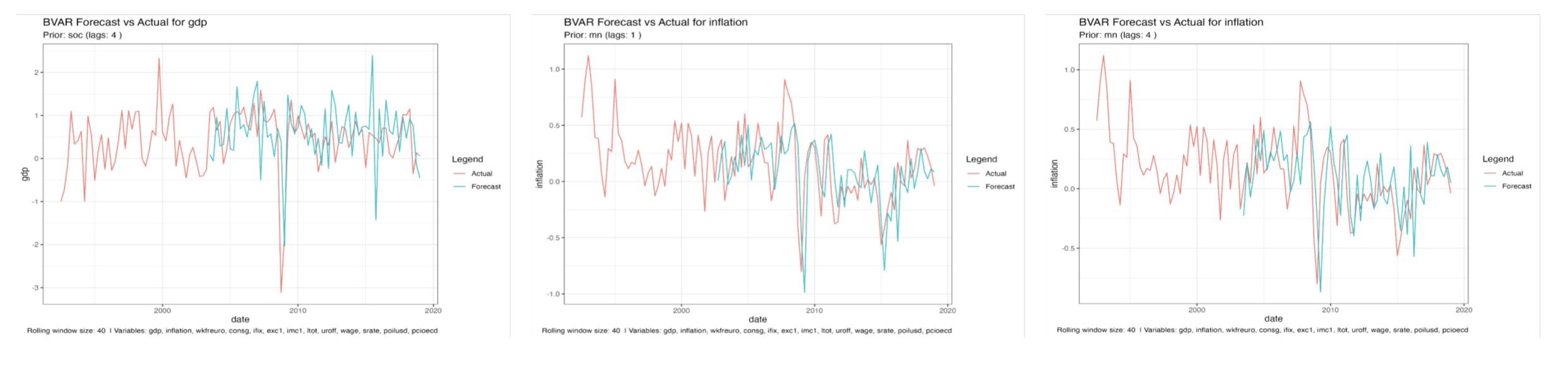

Different window sizes in BVAR

Different window sizes.

In this section, we also tested for different rolling window sizes and we observed:

Smaller windows → higher variance and wider prediction bands
Larger windows → smoother predictions but less sensitivity

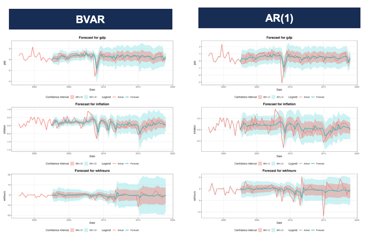
5. Comparison with AR and VAR

We also compared the forecasting performance of BVAR, OLS-VAR and a simple AR(1) using rolling-window MRSE and the Log Score on the training data. The aggregated MRSE by target variable is shown below.

variable	rmse_bvar	rmse_var	rmse_ar1
gdp	0.668	0.677	0.659
inflation	0.284	0.290	0.288
wkfreuro	2.667	2.702	2.635

Why AR(1) is often surprisingly accurate:

Simplicity: AR(1) captures short-term autocorrelation without adding estimation noise.
Weak short-run cross-effects: short-horizon interactions between macro variables are often weak or unstable.
Overfitting risk: multivariate models can add variance that offsets potential gains from modeling cross-variable dynamics.

AR and BVAR comparison

6. Forecasting with the best configuration

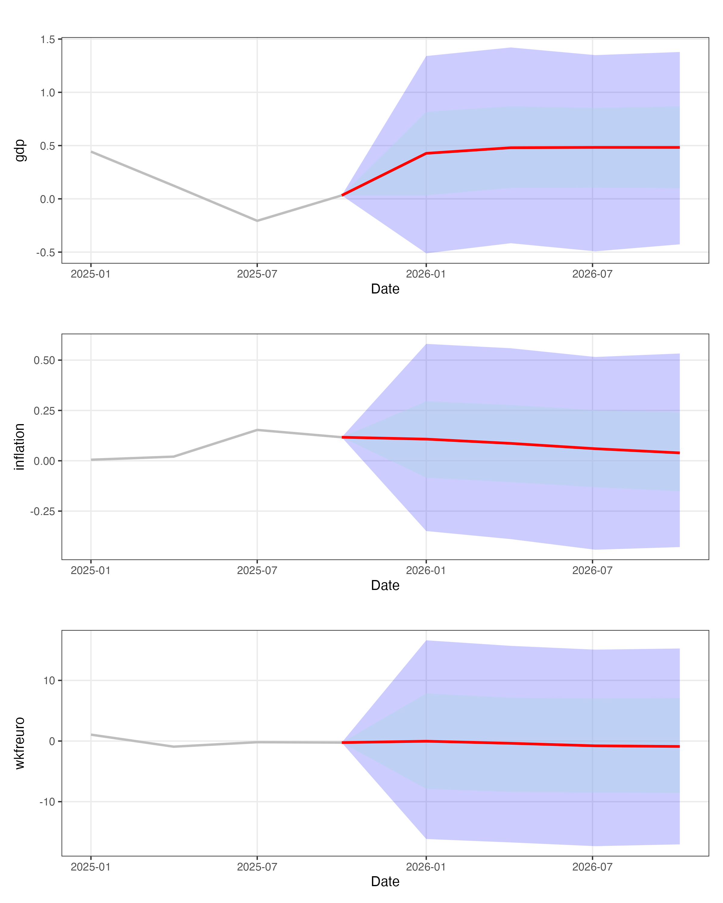
We then picked the best performing model and made our actual prediction, using training data up to 2019 (to exclude covid) to make a prediction for all the quarters of 2026 (h = 1,2,3,4)

df_fc <- df_fc %>% filter(date <= as.Date("2025-10-01")) 

horizon <- 4
window_data <- df[(nrow(df)-40):nrow(df), ]
y_train <- window_data

trained_model <- bvar(
  y_train %>% dplyr::select(all_of(selected_variables)),
  lags = lag_number,
  n_draw = 10000,
  n_burn = 2500,
  n_thin = 1,
  priors = priors,
  verbose = FALSE
)

n_obs <- nrow(df_fc) + horizon  

pred_q50  <- matrix(NA_real_, nrow = n_obs, ncol = length(selected_variables),
                    dimnames = list(NULL, selected_variables))
pred_q16  <- pred_q50
pred_q84  <- pred_q50
pred_q025 <- pred_q50
pred_q975 <- pred_q50

# --- model prediction with BVAR ---------------------------------------------------------
prediction <- predict(trained_model, horizon = horizon, newdata = df_fc[,selected_variables], conf_bands = c(0.16, 0.025))

Then we plotted median forecasts and predictive intervals (quantiles) for each variable to show point predictions together with forecast uncertainty.

A comparison with the KOF (Swiss Economic Institute) forecasts is possible (their public forecasts are available at konjunkturprognose.kof.ethz.ch), but we didn not include it here because their methodology is not fully disclosed.

BVAR Forecast

Different window sizes.

Conclusion and discussion

Our experiments show that BVARs are a practical solution to the overparameterization problem that plagues large OLS-VAR systems: informative priors (e.g., Minnesota) stabilise estimation and typically yield more reliable density forecasts in small samples. At short horizons, however, a simple AR(1) often remains a very competitive model.

To sum up:

BVAR (with informative priors) is preferable when the system size is large relative to the sample, a probabilistic (density) forecasts or credible intervals are needed or priors encode useful economic information.
AR(1) is a robust, low-variance baseline for short-term point forecasts and should be included in any forecasting comparison.
OLS-VAR can underperform due to overfitting when there are many coefficients relative to observations.

However, the model uses training data up to 2019 and excludes explicit scenario analysis for external shocks or structural breaks (e.g., COVID, policy regime changes). Including post‑COVID observations and structural-break tests would help assess robustness.

Bibliography

Lecture Notes from Methods for Macroeconomic Forecasting
GitHub Course Repository
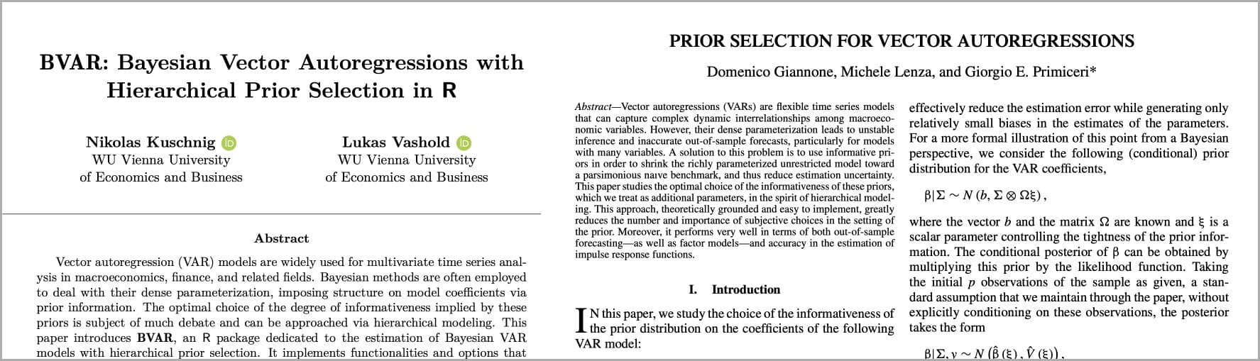
BVAR: Bayesian Vector Autoregressions with Hierarchical Prior Selection in R, Nikolas Kuschnig, Lukas Vashold
Prior Selection for Vectore Autoregression, Domenico Giannone, Michele Lenza, and Giorgio E. Primiceri
Stationarity and Differencing
Forecasting: Principles and Practise
Grok AI (code review)
ChatGPT 5 (code review)