These notes are freely taken from the book Machine Learning for Asset Managers (Elements in Quantitative Finance). They are often incomplete and not 100% accurate, as I intentionally skipped mathematical proofs and focused mostly on the practical concepts.

Index

1. Introduction
2. Denoising and Detoning
3. Distance Metrics
4. Optimal Clustering
5. Financial Labels
6. Feature Importance Analysis
7. Portfolio Construction
8. Testing Set Overfitting
9. Bibliography

1. Introduction

Why Not to Do Backtesting

Contrary to popular belief, backtesting is not a research tool.
Backtests can never prove that a strategy is a true positive.

Never develop a strategy just because of backtests.
Strategies must be supported by theory, not only historical simulations.

Your theories must be general enough to explain particular cases, including extreme events (black swans).

Role of Machine Learning (ML)

• ML helps discover hidden variables.
• ML itself does not reveal the relations between variables. Therefore:
  • Formulate a theory that binds the elements together.
  • Test the theory in different contexts (even where ML found no signal).

Once the theory has been tested, it should stand on its own.
The theory, not the ML algorithm, should make predictions.

Uses of ML

• Existence: ML can indicate the presence of previously unknown relations by predicting outcomes.
• Importance: Feature-importance measures reveal which variables matter more for model performance.
• Causation: ML can support causal inference by comparing predictions.
• Reductionism: Dimensionality reduction can reveal low-dimensional structure and clusters.
• Retrieval: ML scans large datasets to find rare events.
• Outlier Detection: ML identifies anomalies using learned patterns.

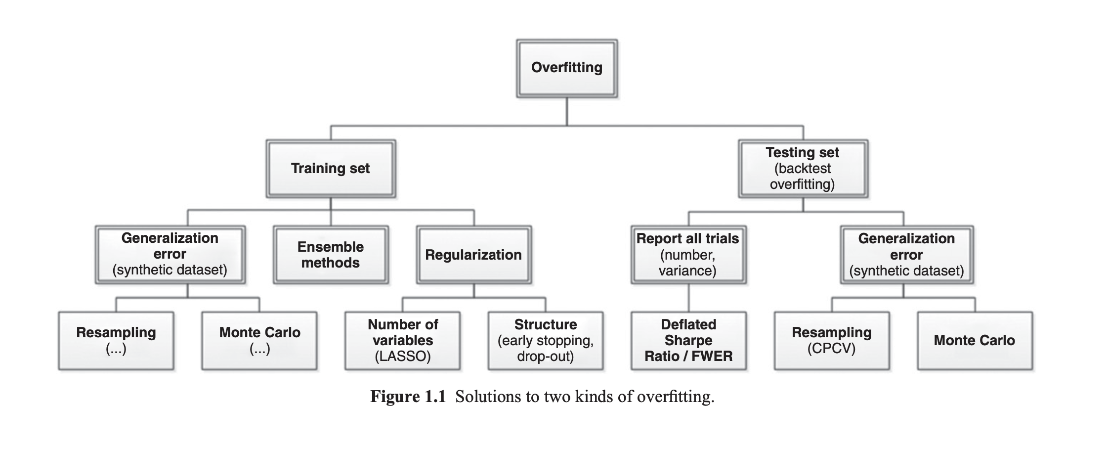
Types of Overfitting

• Train-set overfitting: model fits noise and signal in the training data (learns tiny irrelevant movements).
• Test-set overfitting: repeatedly testing many models on the same test set and selecting the best-performing one.

A useful diagnostic is the generalization gap:

where $E_{\text{train}}$ and $E_{\text{test}}$ are the expected errors (or loss) on training and test sets respectively. A large positive $G$ indicates overfitting.

2. Denoising and Detoning

Covariance Matrix

Covariance matrices are empirically obtained, so they contain a significant amount of noise.
If used directly (e.g., for portfolio optimization), this noise can make results unstable.

The theorem tells us what the eigenvalues of a covariance (or correlation) matrix should look like if the data is completely random.

• If we compute the covariance matrix of asset returns, some of the eigenvalues may just be noise. (random correlations that don’t carry information).

Consider a matrix $X\in {\mathbb{R}}^{T\times N}$ with:

• $T$ observations (rows)
• $N$ assets (columns)

Assume returns have mean $0$ and variance ${\sigma }^2$. Compute the sample covariance matrix:

Each eigenvalue $\lambda$ represents how much variance is explained by a certain “direction” (or factor) in the data.

If the data is purely random, the eigenvalues follow a known distribution: the Marčenko–Pastur distribution.

The theorem tells us that the eigenvalues will lie between two limits:

All eigenvalues between ${\lambda }_{-}$ and ${\lambda }_{+}$ are what we expect from random data, they are just noise .
Eigenvalues larger than ${\lambda }_{+}$ (or smaller than ${\lambda }_{-}$) may represent true correlations or factors in the data.

The basic Marčenko–Pastur theorem assumes that all eigenvalues are random.

In real financial data, this assumption is not valid, some eigenvalues capture true, non-random structure, such as market factor (the first principal component, representing systematic market risk), sector effects or other common risk factors.

The Solution: Laloux Adjustment

Laloux proposed an approach to adjust the Marčenko–Pastur model to account for the presence of non-random eigenvalues.

1. Identify non-random eigenvalues, typically the largest eigenvalues (e.g., the first one representing the market mode).

2. Remove their contribution from the variance
   • Since these are not random, they should not increase the estimated noise level.
   • Adjust the variance:
   $${\sigma }_{\text{adjusted}}^2={\sigma }^2(1-\frac{{\lambda }_{+}}{N})$$
3. Recompute Marčenko–Pastur bounds
   • Use the adjusted variance to compute new limits:
   $${\lambda }_{-}={\sigma }_{\text{adjusted}}^2(1-\sqrt{\frac{N}{T}}{)}^2,{\lambda }_{+}={\sigma }_{\text{adjusted}}^2(1+\sqrt{\frac{N}{T}}{)}^2$$
4. Fit the theoretical PDF
   • Fit the Marčenko–Pastur distribution wit updated data to estimate how much variance is explained by random noise.

Denoising

When you build a correlation matrix from asset returns, a lot of its eigenvalues come from noise.

If you use this noisy matrix directly (e.g. in portfolio optimization), the results are unstable and misleading.

So, the idea is to denoise the matrix: keep the information from the meaningful eigenvalues (the big ones above the Marčenko–Pastur threshold) and replace the noisy ones with something cleaner.

1. Decomposition of the denoised correlation matrix

Start from the denoised correlation matrix $C_1$ with its eigen-decomposition:

where $W=[w_1,\dots ,w_N]$ (orthonormal eigenvectors) and $\Lambda =\mathrm{diag}({\lambda }_1,\dots ,{\lambda }_N)$.

Partition the eigenpairs into market components (hopefully justone, typically the largest eigenvalue(s)) and non-market (detoned) components.

so that

2. Remove the market (detoning)

Subtract the market part to get the detoned correlation matrix $C_2$:

Because we removed at least one eigenvector, $C_2$ is singular (it has at least one zero eigenvalue).

Rescale to enforce unit diagonal if you need a correlation matrix:

3. Portfolio optimization in the reduced (principal-component) space

You cannot directly invert $C_2$. Instead optimize on the non-zero principal components (the detoned subspace) and then map allocations back to the original assets.

Write a portfolio as a linear combination of the surviving eigenvectors:

where $W_{+}$ is the matrix of eigenvectors that survived detoning (i.e. the columns of W_D), and $f$ is the vector of allocations on those principal components.

Take the classic mean–variance objective (risk aversion $\gamma$):

Substitute $\omega =W_{+}f$. Using orthonormality and the block decomposition, the objective in $f$ becomes

where ${\Lambda }_{+}$ is the diagonal matrix of the non-zero eigenvalues (the same as ${\Lambda }_D)$.

The first-order optimality condition yields the closed form

Finally map back to original asset weights:

Note: because W_+ columns are orthonormal, $W_{+}^{\top }$ is the left-inverse of $W_{+}$. This expression avoids inverting the full (singular) $C_2$ and only requires inverting the diagonal ${\Lambda }_{+}$.

What is $f$?

So $f_i$ tells you how much you are investing in eigenportfolio i (the eigenportfolio built from eigenvector $w_i$).

After detoning (removing market eigenvectors), we only keep the “surviving” eigenvectors $W_{+}$. Instead of trying to optimize in the full asset space, we solve for $f$ in the reduced space:

Then we map back to original asset weights:

This way we only allocate risk to components that carry non-noise information.

Shrinkage

Shrinkage is a technique to improve the estimation of covariance (or correlation) matrices when data is noisy or limited.

Empirical covariance matrices, estimated from historical returns, are often unstable or ill-conditioned (especially if you have many assets and few observations). So, instead of using the raw covariance matrix $C_{\text{empirical}}$, combine it with a target $C_{\text{target}}$ that is more stable (like the identity matrix or an average correlation matrix).

Formally:

$\alpha \in [0,1]$ = shrinkage intensity.

• $\alpha =0$ : no shrinkage (use raw covariance)
• $\alpha =1$ : full shrinkage (use only the target)

3.Distance Metrics

Correlation

Correlation $\rho [X,Y]$ measures linear codependence but is not a metric (fails nonnegativity and triangle inequality).

We therefore need a metric that gives a geometry/topology to compare and cluster data, so define:

$d_{\rho }[X,Y]$ standardize X,Y into zero-mean, unit-variance vectors x,y.

If we look at the Euclidean distance:

it expands to:

So $d_{\rho }$ is proportional to a Euclidean distance, hence inherits metric properties.

$d_{\rho }\in [0,1]$ since $\rho \in [-1,1]$.

Positively correlated show small distance, negatively correlated large distance.
This makes sense in long-only portfolios (negatively correlated assets act as diversifiers).

Absolute Correlation

Sometimes, in long-short portfolios, we want negatively correlated assets to be considered similar.

So we can define absolute correlation by:

That is still a metric but highly negatively correlated assets have small distance.

Problems of Correlation

• Correlation quantifies the linear codependecyof two assets
• It’s highly influenced by outliers
• Its application beyond the multivariate Normal case is questionable (In the Gaussian world correlation is a clean, sufficient measure of dependence, outside it correlation can be unstable, incomplete, or misleading).

So better to introduce other metrics.

Entropy of a Discrete Random Variable

Shannon entropy measures the average amount of information needed to describe the outcome of a random variable or the uncertainty or diversification

For random variable $X$ with support $S_X$ and pmf $p(x)$:

with the convention that: $0\log 0:=0$ (limit argument).

If event $x$ has probability $p(x)$, its “surprise” is $\frac{1}{p(x)}$, so low probability brings high surprise.

Entropy can be interpreted as the expected surprise: it's the average uncertainty in $X$.

When all probability mass is on a single outcome, there's no uncertainty and $H(x)=0$. The Maximum entropy is reached when $X$ is uniform over its support and has

Joint Entropy

For random variables $X$, $Y$ with joint pmf $p(x,y)$:

It measures the uncertainty of the pair $(X,Y)$ considered together.

Propertries:

• $H(X,Y)=H(Y,X)$

• $H(X,X)=H(X)$

• $H(X,Y)\ge \max \{H(X),H(Y)\}$

• $H(X,Y)\le H(X)+H(Y)$

(equality holds if $X$ and $Y$ are independent.)

Conditional Entropy

The conditional entropy of $X$ given $Y$ is:

$H(X|Y)$ measures the remaining uncertainty about X once Y is known.

• Conditional entropy is always ≤ entropy:

• Knowing $Y$ can never increase the uncertainty about X.

• Equality occurs if $X$ and $Y$ are independent ($Y$ gives no info about $X$).

• Entropy of a variable given itself:

If you already know X, there’s no uncertainty left.

• Chain rule for entropy:

Total uncertainty about $(X,Y)$ can be decomposed into uncertainty of $Y$ and residual uncertainty of $X$ after knowing $Y$.

Kullback–Leibler Divergence

For two discrete probability distributions $p$ and $q$ defined on the same set $S_X$:

• $p(x)$ = true probability of x

• $q(x)$ = reference or approximate probability of $x$

• Condition: if $q(x)=0\Rightarrow p(x)=0$ to avoid division by zero

• KL divergence measures how much $p$ diverges from $q$.

• It quantifies the “extra information” required if we encode data using $q$ instead of the true distribution $p$.

• $D_{KL}(p\parallel q)\ge 0$ Equality occurs only when $p=q$.

• $D_{KL}(p\parallel q)\ne D_{KL}(q\parallel p)$ (Order matters, so KL divergence is not a metric)

• Triangle inequality fails, so KL divergence does not satisfy all properties of a distance metric.

• If $q(x)=1/|S_X|$ (uniform distribution),$D_{KL}(p\parallel q)$ measures how far p is from uniform.

Cross Entropy

For two discrete probability distributions $p$ (true distribution) and $q$ (approximation or model) defined on the same set $S_X$:

• $p(x)$ = true probability of outcome x
• $q(x)$ = probability assigned by a model or reference distribution
• It measure the uncertainty of $X$ when using $q$ instead of the true $p$.

Entropy: $H(p)=-\sum p(x)\log p(x)$ measures uncertainty using the true distribution.

Cross-entropy: $H(p,q)=H(p)+D_{KL}(p\parallel q)$

• Cross-entropy is always greater than or equal to true entropy.
• The difference $H(p,q)-H(p)=D_{KL}(p\parallel q)$ measures how “wrong” $q$ is.

Mutual Information

Mutual information measures how much knowing one variable reduces uncertainty about another.

• $H(X)$ = entropy of $X$ (uncertainty about $X$)
• $H(X|Y)$ = conditional entropy of $X$ given $Y$ Equivalently:

• Non-negative: $I(X;Y)\ge 0$ $MI=0$ if $X$ and $Y$ are independent (knowing $Y$ gives no info about $X$)
• Symmetric: $I(X;Y)=I(Y;X)$
• Upper bound: $I(X;Y)\le \min \{H(X),H(Y)\}$
• Not a metric: Does not satisfy triangle inequality
• Grouping / decomposition:
  $$I(X;Y;Z)=I(X;Y)+I((X,Y);Z)$$

Mutual information can be expressed as a KL divergence:

It measures >how far the joint distribution is from independence.

4. Optimal Clustering

Clustering groups objects (items) by similarity using their features. The goal is to produce clusters where intra-cluster similarity is high and inter-cluster similarity is low. Clustering is a form of unsupervised learning because we do not provide labelled examples.

Proximity matrix

A proximity matrix measures how "close" or "similar" objects in a dataset are to each other.

• For a dataset with $n$ elements, the proximity matrix $P$ is an $n\times n$ matrix.
• Each entry $P[i,j]$ represents the closeness between object $i$ and object $j$.

Typical definitions:

• $P[i,j]=\text{similarity}(x_i,x_j)$
• $P[i,j]=\text{distance}(x_i,x_j)$

A symmetric proximity matrix with zeros on the diagonal is common when using pairwise distances.

Two main families of clustering:

Hierarchical clustering

• Produces a nested sequence of partitions (a dendrogram).
• Top: a single cluster containing all points. Bottom: each point alone.
• Two approaches:
  • Agglomerative (bottom-up): start with a lot of partitions and merge.
  • Divisive (top-down): start with one cluster and split.
• No need to specify $K$ up-front (but you choose a cut in the dendrogram to get $K$ clusters).

Partitional clustering

• Partitions the dataset into $K$ disjoint clusters.
• Each object belongs to exactly one cluster.
• Example: k-means, k-medoids, spectral clustering.
• Often requires the number of clusters $K$ as input.

Practical issues

• Curse of dimensionality: when the number of features is large relative to observations, distances become less informative and clustering can degrade. Dimensionality reduction (PCA, t-SNE, UMAP) or feature selection helps.
• Initialization randomness: algorithms like k-means are sensitive to initial centroids.

Because partitional methods require $K$, several methods exist to estimate a good $K$:

Elbow method

• Compute within-cluster sum of squared errors (WCSS) for different $K$.
• Plot WCSS vs $K$. The "elbow" point (where marginal gain drops) is a reasonable $K$.

Silhouette analysis

• Measures how well each point lies within its cluster compared to the nearest other cluster.

For an observation $i$:

• Let $a_i$ = average distance from $i$ to all other points in the same cluster (intra-cluster distance).
• Let $b_i$ = minimum over other clusters of the average distance from $i$ to points in that other cluster (nearest inter-cluster distance).

The silhouette coefficient for $i$ is

• $S_i\approx 1$: well clustered (close to own cluster, far from others).
• $S_i\approx 0$: on or near cluster boundary.
• $S_i<0$: likely misclassified (closer to another cluster).

The average silhouette score across all points is a scalar summary used to compare different $K$: higher is better.

Practical checklist for clustering

1. Preprocess
   • Standardize / normalize features when distances are used.
   • Handle missing values.
   • Reduce dimensionality if needed.
2. Choose distance / similarity
   • Euclidean for continuous, cosine for directional data, Jaccard for binary sets, etc.
3. Choose algorithm
   • Hierarchical if you want a dendrogram and no fixed $K$.
   • K-means/k-medoids for large datasets with spherical-ish clusters.
4. Select $K$
   • Use elbow, silhouette, gap statistic, or domain knowledge.
5. Validate
   • Visual inspection (2D/3D embedding).
   • Cluster compactness and separation metrics (silhouette, Davies–Bouldin).
   • If possible, external validation against known labels.

Once we run a clustering algorithm (e.g., k-means), we still need to evaluate how good the clustering result is.

Quality Measure $q$

Define the overall clustering quality:

Where:

• $E[S_i]$ = mean of silhouette scores (average clustering quality).
• $V[S_i]$ = variance of silhouette scores (consistency across points).

Higher $q$ means better clustering (high average silhouette, low variability).

Base Clustering Algorithm

At the base level, the procedure works as follows:

1. Input
   • Start from the observation (distance/similarity) matrix.
2. Outer Loop (over $K$)
   • For $k=2,3,\dots ,N$:
     • Run k-means clustering with $k$ clusters.
     • Compute the quality measure $q$ from silhouette scores.
     • Store results for that $k$.
3. Inner Loop (over initializations)
   • Repeat the above with different random initializations of centroids.
   • This reduces sensitivity to random starts.
4. Selection
   • Choose the clustering result with the highest quality $q$.
   • This yields:
     • Optimal number of clusters $K$.
     • Best initialization (most stable clustering result).

Even after selecting the best $K$ and initialization, some clusters can still be poor quality.

Reclustering Low-Quality Clusters

To refine the clustering, we recluster only the bad clusters.

1. Start with Base Clustering Result
   • We already have $K$ clusters from the base algorithm.
   • For each cluster $k$, compute its quality score $q_k$ (mean silhouette score of its members).
2. Identify Poor-Quality Clusters
   • Compute overall average quality:
     $$q=\frac{1}{K}\sum _{k=1}^K{q}_k$$
   • Identify clusters with $q_k<q$ → “below-average quality.”
   • Let $K_1$ = number of such clusters.
3. Decision Rule Based on $K_1$

• If $K_1\le 1$:
  • No meaningful reclustering, so return base clustering.
• If $K_1\ge 2$:
  • Recluster only those $K_1$ clusters :
    • Build a new observation matrix for elements of these clusters.
    • Rerun the base algorithm (search over $K$ and initializations) on this reduced subset.

4. Check Improvement
   • Compare average quality before vs. after reclustering.
   • If quality improved:
     • Merge the unchanged good clusters with the newly reclustered clusters.
   • Else:
     • Keep the original base clustering result.

5. Financial Labels

Supervised learning aims to predict an output $y$ given features $X$.

Types of Supervised Learning

• Regression problems
  • Predict a continuous target (real numbers).
  • Examples drawn from infinite population (countable like integers or uncountable like reals).
• Classification problems
  • Predict a discrete label from a finite set (e.g., $0,1$, $bearish,bullish$).

Fixed-Horizon Labeling

We have a feature matrix:

• $X=\{X_i{\}}_{i=1}^I$
• For each observation $X_i$:
  • Let $t_{i,0}$ = index of bar where features are sampled.
  • Define a fixed horizon $h$.
  • Compute return over horizon $h$:

Assign label $y_i\in \{-1,0,1\}$ based on return:

Where:

• $\tau$ = constant return threshold.
• Time bars = bars sampled at regular time intervals.
• Result: fixed time horizons for all samples.

Concerns with Fixed-Horizon Labeling

• Returns show intraday volatility patterns (open/close more volatile).
• Constant $\tau$ transfers seasonality into labels, label distribution becomes non-stationary.

Solution: use tick/volume/dollar bars instead of time bars or standardize returns using volatility estimate:

where ${\sigma }_{t_{i,0};t_{i,1}}$ = predicted volatility. Then apply labeling rule to $z$-scores.

Triple-Barrier Method

Labels should represent actual trading outcomes: profit, loss, or timeout.

This method sets three barriers:

1. Upper Horizontal Barrier: Profit-taking (success).
2. Lower Horizontal Barrier: Stop-loss (failure).
3. Vertical Barrier: Maximum holding period (timeout).

Step-by-Step Procedure

1. Start at $t_{i,0}$ (where features $X_i$ observed).
2. Monitor price path forward until one barrier is hit.
3. Assign label $y_i$:
   • If upper barrier reached first: $y_i=+1$.
   • If lower barrier reached first: $y_i=-1$.
   • If vertical barrier reached first:
     • Option 1: $y_i=0$ (neutral).
     • Option 2: $y_i=\text{sgn}(r_{t_{i,0};t_{i,1}})$ (final return sign).

Trend Scanning Method

Instead of setting a fixed horizon $h$, profit-taking, or stop-loss levels, trend scanning lets trends run naturally until they end.

Label each observation as part of:

• Uptrend: $y_t=+1$
• Downtrend: $y_t=-1$
• No trend: $y_t=0$

Define a Trend

Fit a local linear regression over a window of $L$ observations:

• ${\beta }_1$ = slope, direction & strength of trend.
• ${\epsilon }_{t+l}$ = residuals (noise).

Test Statistical Significance

Compute t-statistic of the slope:

• Large $|{\hat{t}}_{{\beta }_1}|$: strong trend evidence.
• Near 0: no clear trend.

Assign Labels

For each $t$:

Where $\tau$ = critical t-value threshold.

Meta-Labeling

Meta-labeling is a two-model approach:

1. Primary model: predicts position direction (long/short).
2. Secondary (meta) model: predicts whether that position will be profitable (filtering false positives).

The goal is to reduce exposure to losing trades and size positions proportionally to predicted success probability.

Expected Value & Risk

Let $p$ = probability of profit and $\pi$ = payoff magnitude.

The expected value is:

• $p>0.5\Rightarrow \mu >0$: positive expected profit.
• $p=0.5\Rightarrow \mu =0$: no edge.

Expected Variance

• Highest when $p=0.5$ (most uncertain).
• Shrinks as $p\to 0$ or $1$ (certainty increases).

Sharpe Ratio

Standardize risk/return with Sharpe-like measure:

• $z>0$: attractive opportunity.
• $z<0$: avoid trade.

Mapping to Position Size

Convert $z$ to position size $m\in [-1,1]$:

Where $Z(\cdot )$ = CDF of standard normal.

• $z=0\Rightarrow m=0$ (no trade)
• Large $z>0\Rightarrow m\to 1$ (max long)
• Large $z<0\Rightarrow m\to -1$ (max short)

Meta-Labeling for Position Size with Multiple Classifiers

Suppose we have $n$ meta-labeling classifiers:

Sum of predictions:

• Mean: $E[\sum y_i]=np$
• Variance: $Var[\sum y_i]=np(1-p)$

As $n\to \infty$, by de Moivre–Laplace :

Thus, average prediction:

Hypothesis Test

Null hypothesis: $H_0:p=0.5$ (no predictive edge)

t-statistic:

Follows Student-t distribution with $n-1$ d.o.f.

Mapping t to Bet Size

Convert $t$ to bet size $m\in [-1,1]$:

Where $T_{n-1}(\cdot )$ = CDF of Student-t distribution.

• $t=0\Rightarrow m=0$ (no bet)
• Large $t>0\Rightarrow m\to 1$ (max long)
• Large $t<0\Rightarrow m\to -1$ (max short)

In practical:

• $\hat{p}\to 1$: strong long conviction → large $m>0$.
• $\hat{p}\to 0$: strong short conviction → large $m<0$.
• $\hat{p}\approx 0.5$: no edge → $m\approx 0$ (no position).

6. Feature Importance Analysis

P-Values (Statistical Significance)

Probability of observing the estimated coefficient if the true coefficient = 0 .

It tests whether a feature has any effect, not its predictive power.

The p-value is a probability, but not the probability that your hypothesis is true. It answers a very specific question:

“If the null hypothesis were true, how likely is it to observe a result as extreme (or more extreme) than what I actually observed?”

• False positives/negatives if model assumptions fail.
• Not robust with multicollinearity (correlated features).
• Measures statistical relevance, not:
  • Effect size
  • Predictive power
  • Causality

A low p-value doesn't mean feature is “important”, it only means the effect is statistically detectable.

Mean Decrease Impurity (MDI) — Tree-Based Models

A clear video explanation can be found here, credits to StatQuest

1. At each node pick feature $X_f$ and threshold $\tau$ to split:
   • Left: $X_f<\tau$
   • Right: $X_f\ge \tau$
2. Measure impurity with e.g.:
   • Entropy: $H(t)=-{\sum }_c{p}_c{\log }_2{p}_c$
   • Gini: $G(t)=1-{\sum }_c{p}_c^2$
3. Information gain (impurity reduction) for a split:
   $$\Delta g(t,f)=i(t)-\frac{N(t_0)}{N(t)}i(t_0)-\frac{N(t_1)}{N(t)}i(t_1)$$
4. Feature importance (MDI) for feature $f$: sum of weighted $\Delta g(t,f)$ over all nodes where $f$ was used.

Mean Decrease Accuracy (MDA)

This algorithm measures out-of-sample importance.

1. Fit model and compute cross-validated performance (baseline).
2. For each feature:
   • Shuffle that feature's values (breaks relationship with target).
   • Recalculate cross-validated performance.
3. $MDA$ = performance(before shuffle) − performance(after shuffle).

• Large positive MDA means that feature important.
• MDA near zero means that feature irrelevant.
• Negative MDA means feature damaging performance (model improved after shuffling).

Model Performance Metrics

Negative Average Likelihood (NegAL)

where $y_{n,k}=1$ if observation $n$ has true label $k$, else 0; $p_{n,k}$ is predicted prob.

Range:$0\le \text{NegAL}\le 1$.
Higher =is better (closer to 1 the model assigns higher probability to true labels).

Probability-Weighted Accuracy (PWA)

where $y_n=1$ if prediction correct else 0; $p_n={\max }_k{p}_{n,k}$.

It weighs correct predictions by model confidence.

Feature Clustering for Importance

With highly codependent features the individual importance unreliable, so it's commonoto cluster features to analyze them better.

1. Represent features in a metric space
   • Options:
     • Correlation-based distances (linear dependencies).
     • Information-theoretic metrics (e.g., Variation of Information) to capture nonlinear redundancies.
2. Cluster formation
   • Apply an ONC (Optimal Number of Clusters) algorithm:
     • Finds number of clusters and assignments.
     • Partitional assignment: each feature belongs to exactly one cluster.
     • Within-cluster features share much information; across clusters share little.
3. Optional residualization
   • For cluster $k$, regress each feature $X_{n,i}\in D_k$ on features from earlier clusters ${\cup }_{l<k}{D}_l$:
     $$X_{n,i}={\alpha }_i+\sum _{j\in {\cup }_{l<k}{D}_l}{\beta }_{i,j}{X}_{n,j}+{\epsilon }_{n,i}$$
   • Replace $X_i$ with residuals ${\hat{\epsilon }}_i$.
   • If regressors are too many, reduce dimensionality inside clusters.

• Apply MDI or MDA at the cluster level (not single-feature).
• Interpret which groups of features drive model performance.

7. Portfolio Construction

Given $N$ assets the expected excess returns $\mu$ (vector $N\times 1$) and the covariance matrix $V$ ($N\times N$), the goal is to find portfolio weights $\omega$ that minimize portfolio variance .

Classical Mean–Variance Optimization (Variance Minimization)

The vector $a$ encodes the portfolio constraint (e.g., fully invested: $a=1_N$).

Lagrangian:

Useful Special Cases

• Equal weights under isotropic variance: $a=1_N,V={\sigma }^2{I}_N$, ${\omega }^{\ast }=\frac{1}{N}{1}_N$
• Inverse-variance : $a=1_N,V$ diagonal, ${\omega }_n^{\ast }\propto \frac{1}{V_{n,n}}$
• Minimum-variance: $a=1_N$, ${\omega }^{\ast }=\frac{V^{-1}{1}_N}{1_N^{\top }{V}^{-1}{1}_N}$
• Maximum Sharpe : $a=\mu$, ${\omega }^{\ast }=\frac{V^{-1}\mu }{1_N^{\top }{V}^{-1}\mu }$

Numerical Stability & Conditioning Problem

Let $C$ be the standardized correlation matrix of $V$. The solution needs to calculate on $V^{-1}$.

If assets are highly correlated ($|\rho |\approx 1$), then $C$ is ill-conditioned:

• Condition number large means that $V^{-1}$ numerically unstable (small errors in $V$ estimate produce large swings in $V^{-1}$). We need Markowitz when correlations exist, but those same correlations make the solution unstable.

Practical fixes :

• Shrinkage estimators (Ledoit–Wolf)
• Factor models (lower-dimensional structure)
• Regularization: add $\delta I$ to $V$ before inversion ($V+\delta I$)
• Robust/resampled optimization, constraints on weights (box, turnover), or use of priors (Black–Litterman)

Nested Clustered Optimization (NCO)

The goal is tos tabilize Markowitz by solving smaller, better-conditioned subproblems.

1. Cluster the correlation matrix to find groups of highly correlated assets.
2. Intracluster optimization:
   • For each cluster, compute intracluster weights using the denoised covariance (call it cov1).
   • Smaller cluster size means better-conditioned covariance estimates.
   • With very correlated cluster, the min-variance tends toward equal weights, so instability is limited.
3. Intercluster optimization :
   • Build reduced covariance (cov2) between clusters.
   • cov2 is by construction close to diagonal; invertibility and conditioning are much improved.
4. Combine:
   • Final asset weights = (intra-cluster weights) × (inter-cluster weights).

• Dimensionality reduction: each inversion is on smaller matrices.
• Denoising at step 1 reduces noisy eigenvalues.
• Aggregation produces a near-diagonal inter-cluster covariance, improving stability.

8. Testing Set Overfitting

Selection Bias under Multiple Testing (SBuMT)

SBuMT occurs when a researcher tests many strategies on the same historical dataset and then reports only the best-performing one.

This process leads to false discoveries , strategies that look profitable in-sample but fail in live trading.

True vs. False Investment Strategies & Precision/Recall

The total number of strategies is

where:

• $s_T$ = number of true strategies (positive expected return)
• $s_F$ = number of false strategies (zero or negative expected return)

The Odds ratio of true to false strategies is:

In finance, signal-to-noise ratio is usually very low, meaning most strategies are false.

So the number of true strategies is:

and the number of false ones:

Statistical Errors

• False Positive Rate (Type I error): $\alpha$

  • False Positives (FP): $FP=\alpha s_F$
  • True Negatives (TN): $TN=(1-\alpha )s_F$

• False Negative Rate (Type II error): $\beta$

  • False Negatives (FN): $FN=\beta s_T$
  • True Positives (TP): $TP=(1-\beta )s_T$

The Precision (Positive Predictive Value) is defined as:

and the Recall (Sensitivity) as:

Precision strongly depends on odds ratio θ.

A discovered strategy is more likely to be false than true if:

Type $I$ Error Across Multiple Trials

(False alarm: see a signal where none exists, identify a false positive)

In a single trial :

• $P$(Type I error) = $\alpha$
• $P$(No Type I error) = $1-\alpha$

with K independent trials:

• $P$(No Type I error in any trial): $(1-\alpha {)}^K$
• $P$(At least one Type I error) = Family-Wise Error Rate (FWER):

FWER increases with K , the more strategies you test, the higher the chance of finding a false positive.

Type $II$ Error Across Multiple Trials

(Missed discovery: fail to detect a true strategy)

In a single trial::

• $P$(Type II error) = $\beta$

with K trialsP(Missing all positives):

• $P$(Type II error) $={\beta }_K={\beta }^K$

As $K\uparrow$:

• ${\alpha }_K\uparrow$ (false positive risk grows)
• ${\beta }_K\downarrow$ (less likely to miss all true positives)

Precision & Recall Adjusted for Multiple Testing

The Adjusted Precision can be defined as:

and the Adjusted Recall as:

As $K$ increases:

• Recall improves (lower chance of missing all true strategies).
• Precision usually drops (higher risk of including false positives).

The Sharpe Ratio Framework

Given the strategy excess returns:

and the Population (true) Sharpe Ratio:

The Sample (estimated) Sharpe Ratio is defined as:

where $\bar{r}$ is sample mean return, $s_r$ sample standard deviation.

The distribution of Sample SR can be defined as following.

Case 1: IID Normal Returns

Case 2: Non-Normal Returns

Empirical evidence: hedge fund returns often exhibit:

• Negative skewness
• Positive excess kurtosis

where:

• ${\gamma }_3$ = skewness
• ${\gamma }_4$ = kurtosis

Special case: for Normal returns (${\gamma }_3=0,{\gamma }_4=3$), we recover the initial formula.

SBuMT and Maximum Sharpe Ratios

Given $K$ independent strategies with Sharpe ratios:

the Expected Maximum of K Sharpe Ratios

where:

• $Z^{-1}(\cdot )$ = quantile function of standard Normal
• $\gamma \approx 0.5772$ = Euler–Mascheroni constant
• $e\approx 2.718$

The more strategies you try ($K\uparrow$), the higher the expected maximum Sharpe ratio by chance.

So a discovered strategy is likely a false positive unless:

Deflated Sharpe Ratio (DSR)

Adjusts Sharpe ratio for:

• Multiple testing ($K$)
• Sample size ($T$)
• Skewness (${\gamma }_3$) and kurtosis (${\gamma }_4$)

A high DSR brings stronger evidence of true profitability. A low DSR means thatis likely a false discovery

Clustering Strategies & Cluster-Level Returns

N strategies are grouped into $K\ll N$ clusters based on correlations, so it's possible to reduces dimensionality for multiple testing bias.

The aggregate return series for each cluster is:

Weights chosen to minimize cluster variance:

where:

• ${\Sigma }_k$ = covariance matrix of returns within cluster $k$
• $1_k$ = vector of ones of appropriate size

Clustering reduces effective number of trials $(K\ll N)$:

• Lowers false discovery probability
• Produces a more realistic null distribution
• Improves precision of DSR-based significance testing

Bibliography

• Machine Learning for Asset Managers
• StatQuest YouTube Videos
• ChatGPT-5, OpenAI